线性代数之——行图像和列图像

1. 线性方程组的几何解释

线性代数的中心问题就是解决一个方程组，这些方程都是线性的，也就是未知数都是乘以一个数字的。

$\begin{array}{cccc}{\displaystyle }& {\displaystyle x-}& {\displaystyle 2}& {\displaystyle y=1}\\ {\displaystyle 3}& {\displaystyle x+}& {\displaystyle 2}& {\displaystyle y=11}\end{array}$3​x − x + ​22​y = 1y = 11​

针对上面的方程组，如果我们一行一行来看的话，那么第一个方程 $x-2y=1$x−2y=1 表示二维平面的一条直线。点 (1, 0) 是方程的一个解，点 (3, 1) 也是方程的一个解，因此它们都位于这条直线上。

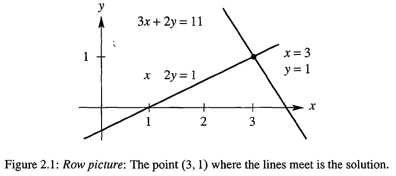
同理，第二个方程 $3x+2y=11$3x+2y=11 也表示二维平面的一条直线，这两条直线的交点也就是上述方程组的解，因为它同时满足了方程一和方程二 。

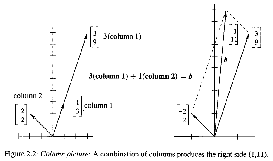
另外，我们也可以将上述方程写成向量的形式：

$x\left[\begin{array}{c}1\\ 3\end{array}\right]+y\left[\begin{array}{c}-2\\ 2\end{array}\right]=\left[\begin{array}{c}1\\ 11\end{array}\right]=b$x[13​]+y[−22​]=[111​]=b

问题就变成了寻找左边两个向量的一个特定线性组合来产生右边的向量。

若将上述方程组表示成矩阵的形式，就是：

$Ax=b\leftrightarrow \left[\begin{array}{cc}1& -2\\ 3& 2\end{array}\right]\left[\begin{array}{c}x\\ y\end{array}\right]=\left[\begin{array}{c}1\\ 11\end{array}\right]$Ax=b↔[13​−22​][xy​]=[111​]

行图像就是对矩阵 $A$A 的行进行处理，而列图像则是矩阵 $A$A 的列的线性组合。

2. 三个未知数三个方程

针对三个未知数 $x,y,z$x,y,z，我们有三个线性方程：

KaTeX parse error: Too many math in a row: expected 2, but got 3

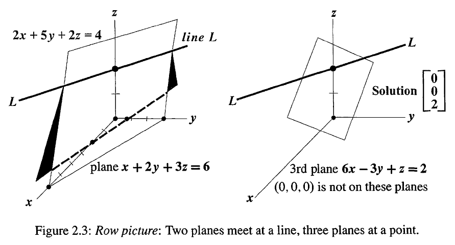
在行图像中，每个方程产生一个三维空间中的平面。第一个平面和第二个平面相交于一条直线 $L$L，然后第三个平面和这条直线又相交于一点，也就是方程组的解。

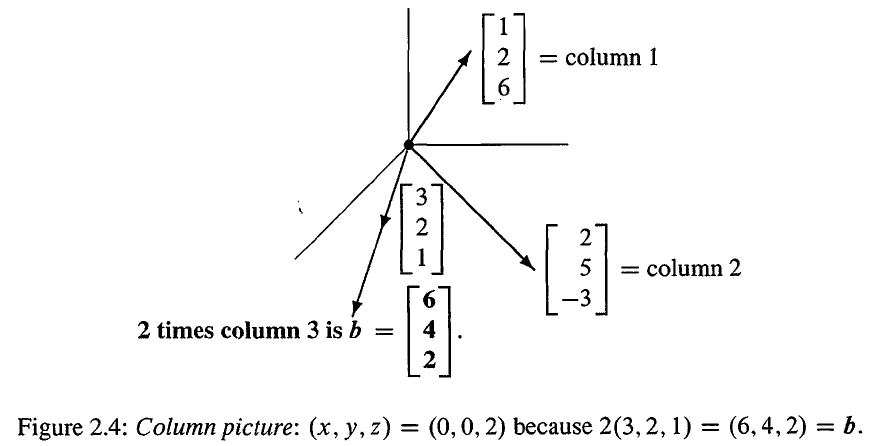
在列图像中，我们要寻找左边向量的一个线性组合。在这里，我们可以非常容易地看到方程组的解，(6, 4, 2) 为 (3, 2, 1) 的 2 倍，因此解就为 (0, 0, 2)。

$x\left[\begin{array}{c}1\\ 2\\ 6\end{array}\right]+y\left[\begin{array}{c}2\\ 5\\ -3\end{array}\right]+z\left[\begin{array}{c}3\\ 2\\ 1\end{array}\right]=\left[\begin{array}{c}6\\ 4\\ 2\end{array}\right]$x⎣⎡​126​⎦⎤​+y⎣⎡​25−3​⎦⎤​+z⎣⎡​321​⎦⎤​=⎣⎡​642​⎦⎤​

表示成矩阵的形式，就是

$Ax=b\leftrightarrow \left[\begin{array}{ccc}1& 2& 3\\ 2& 5& 2\\ 6& -3& 1\end{array}\right]\left[\begin{array}{c}x\\ y\\ z\end{array}\right]=\left[\begin{array}{c}6\\ 4\\ 2\end{array}\right]$Ax=b↔⎣⎡​126​25−3​321​⎦⎤​⎣⎡​xyz​⎦⎤​=⎣⎡​642​⎦⎤​

$A$A 乘以 $x$x 可以看成是 $x$x 和矩阵的行的点积

$Ax=\left[\begin{array}{c}\left(row1\right)\cdot x\\ \left(row2\right)\cdot x\\ \left(row3\right)\cdot x\end{array}\right]$Ax=⎣⎡​(row1)⋅x(row2)⋅x(row3)⋅x​⎦⎤​

也可以看成是矩阵的列的线性组合

$Ax=x\left(column1\right)+y\left(column2\right)+z\left(column3\right)$Ax=x(column1)+y(column2)+z(column3)

获取更多精彩，请关注「seniusen」!