线性代数之——对称矩阵及正定性

当 $A$A 是对称的时候， $Ax=\lambda x$Ax=λx 有什么特殊的呢？

1. 对称矩阵的分解

$A=S\Lambda S^{-1}$A=SΛS−1
$A^T=(S^{-1}{)}^T\Lambda S^T$AT=(S−1)TΛST

如果 $A$A 是对称矩阵，也就是 $A=A^T$A=AT。对比以上两个式子，我们可以得到 $S^{-1}=S^T$S−1=ST，也就是 $S^{T}S=I$STS=I，特征向量矩阵 $S$S 是正交的。

对称矩阵具有如下的性质：

• 它们的特征值都是实数；
• 可以选取出一组标准正交的特征向量。

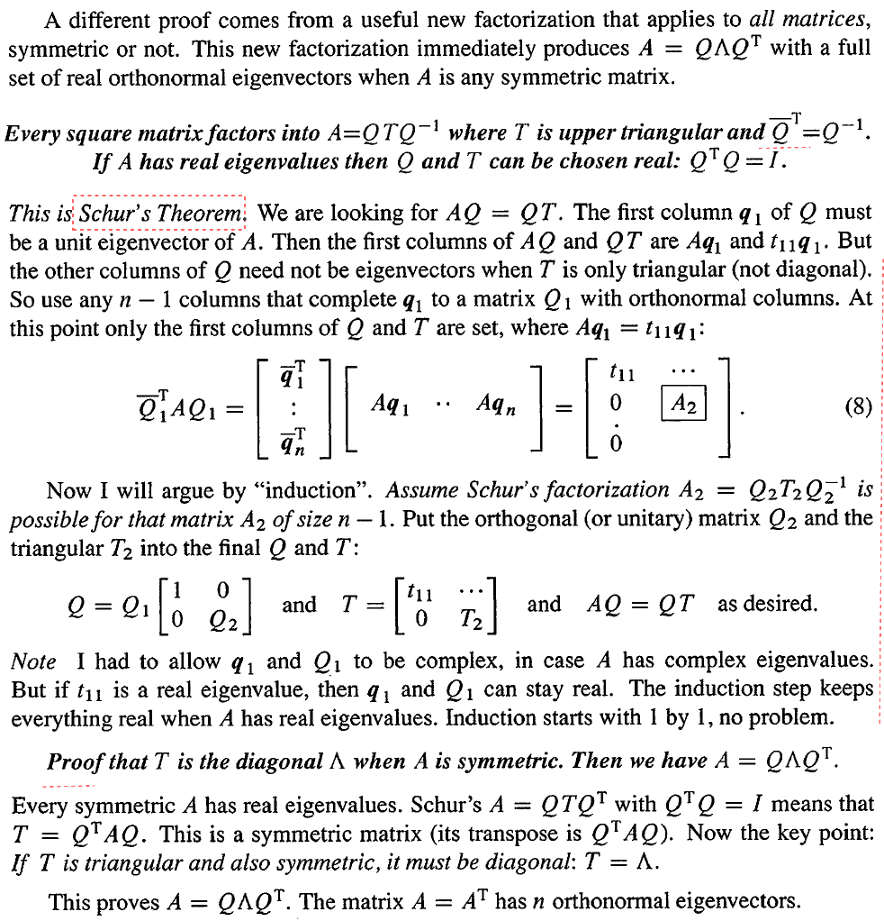
每个对称矩阵都可以分解为 $A=Q\Lambda Q^{-1}=Q\Lambda Q^T$A=QΛQ−1=QΛQT， $\Lambda$Λ 中为实数的特征值， $S=Q$S=Q 中为标准正交的特征向量。

• 例 1

$A=\left[\begin{array}{cc}1& 2\\ 2& 4\end{array}\right]$A=[12​24​]

$A-\lambda I=\left[\begin{array}{cc}1-\lambda & 2\\ 2& 4-\lambda \end{array}\right]$A−λI=[1−λ2​24−λ​]

$det(A-\lambda I)=(1-\lambda )(4-\lambda )-4={\lambda }^2-5\lambda =0$det(A−λI)=(1−λ)(4−λ)−4=λ2−5λ=0

特征值和特征向量分别为：

${\lambda }_1=0，x_1=\left[\begin{array}{c}2\\ -1\end{array}\right]$λ1​=0，x1​=[2−1​]

${\lambda }_2=5，x_2=\left[\begin{array}{c}1\\ 2\end{array}\right]$λ2​=5，x2​=[12​]

特征向量 $x_1$x1​ 位于零空间，特征向量 $x_2$x2​ 位于列空间。有子空间基本定理可知，零空间正交于行空间，这里 $A$A 是对称矩阵，所以列空间和行空间是一样的，因此两个特征向量是垂直的。而要得到标准正交向量，我们只需再除以它们各自的长度即可。所以有：

$Q\Lambda Q^T=\frac{1}{\sqrt{5}}\left[\begin{array}{cc}2& 1\\ -1& 2\end{array}\right]\left[\begin{array}{cc}0& 0\\ 0& 5\end{array}\right]\frac{1}{\sqrt{5}}\left[\begin{array}{cc}2& -1\\ 1& 2\end{array}\right]=A$QΛQT=5 ​1​[2−1​12​][00​05​]5 ​1​[21​−12​]=A

一个实对称矩阵的所有特征值都是实数。

证明

实数的共轭还是它本身，两个数积的共轭等于共轭的积，即 $\overline{AB}=\bar{A}\bar{B}$AB=AˉBˉ。

$\begin{array}{}\text{(1)}& Ax=\lambda x\to \bar{A}\bar{x}=\bar{\lambda }\bar{x}\to A\bar{x}=\bar{\lambda }\bar{x}\end{array}$Ax=λx→Aˉxˉ=λˉxˉ→Axˉ=λˉxˉ(1)

对 (1) 进行转置可得

$\begin{array}{}\text{(2)}& {\bar{x}}^T{A}^T=\bar{\lambda }{\bar{x}}^T\to {\bar{x}}^{T}A=\bar{\lambda }{\bar{x}}^T\end{array}$xˉTAT=λˉxˉT→xˉTA=λˉxˉT(2)

将 $Ax=\lambda x$Ax=λx 乘以 ${\bar{x}}^T$xˉT，将 (2) 式乘以 $x$x，可得

$\begin{array}{}\text{(3)}& {\bar{x}}^{T}Ax=\lambda {\bar{x}}^{T}x\end{array}$xˉTAx=λxˉTx(3)

$\begin{array}{}\text{(4)}& {\bar{x}}^{T}Ax=\bar{\lambda }{\bar{x}}^{T}x\end{array}$xˉTAx=λˉxˉTx(4)

由于右边为向量长度的平方，因此不为零。对比 (3) 、(4) 两式可得 $\bar{\lambda }=\lambda$λˉ=λ，所以对称矩阵的特征值一定为实数。

一个实对称矩阵的所有特征向量（对应于不同特征值）是正交的。

证明

假设有 $Ax={\lambda }_{1}x$Ax=λ1​x 和 $Ay={\lambda }_{2}y$Ay=λ2​y，并且 ${\lambda }_1̸={\lambda }_2$λ1​̸​=λ2​，那么

$({\lambda }_{1}x{)}^{T}y=(Ax{)}^{T}y=x^T{A}^{T}y=x^{T}Ay=x^T{\lambda }_{2}y$(λ1​x)Ty=(Ax)Ty=xTATy=xTAy=xTλ2​y

等式左边为 $x^T{\lambda }_{1}y$xTλ1​y，等式右边为 $x^T{\lambda }_{2}y$xTλ2​y，因为 ${\lambda }_1̸={\lambda }_2$λ1​̸​=λ2​，所以有 $x^{T}y=0$xTy=0，也即两个特征向量垂直。

• 例 2

$A=\left[\begin{array}{cc}a& b\\ b& c\end{array}\right]$A=[ab​bc​]

特征向量分别为：

$x_1=\left[\begin{array}{c}b\\ {\lambda }_1-a\end{array}\right]$x1​=[bλ1​−a​]

$x_2=\left[\begin{array}{c}{\lambda }_2-c\\ b\end{array}\right]$x2​=[λ2​−cb​]

$x_1^T{x}_2=b({\lambda }_2-c)+b({\lambda }_1-a)=b({\lambda }_1+{\lambda }_2-a-c)=0$x1T​x2​=b(λ2​−c)+b(λ1​−a)=b(λ1​+λ2​−a−c)=0

两个特征值的和为矩阵的迹，即对角线元素的和。

我们再来看 $2\times 2$2×2 矩阵分解后的结果

$A=Q\Lambda Q^T=\left[\begin{array}{c}\\ x_1& x_2\\ \end{array}\right]\left[\begin{array}{c}{\lambda }_1\\ & {\lambda }_2\end{array}\right]\left[\begin{array}{c}{x}_1^T\\ x_2\end{array}\right]$A=QΛQT=⎣⎡​x1​ ​x2​​⎦⎤​[λ1​ ​λ2​​][x1T​x2​​]

$A={\lambda }_1{x}_1{x}_1^T+{\lambda }_2{x}_2{x}_2^T$A=λ1​x1​x1T​+λ2​x2​x2T​

扩展到 $n$n 维的情况， $A={\sum }_i^n{\lambda }_i{x}_i{x}_i^T$A=∑in​λi​xi​xiT​，其中每一个 $x_i{x}_i^T$xi​xiT​ 都是投影矩阵， $P=\frac{x{x}^T}{x^{T}x}$P=xTxxxT​，特征向量的长度为 1，所以分母略去了。也就是说，对称矩阵是其特征向量投影矩阵的线性组合。

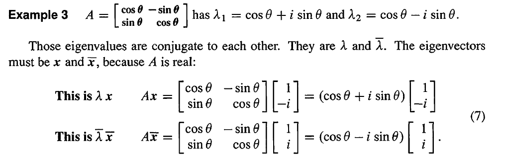
2. 实矩阵的复特征向量

$Ax=\lambda x\to \bar{A}\bar{x}=\bar{\lambda }\bar{x}\to A\bar{x}=\bar{\lambda }\bar{x}$Ax=λx→Aˉxˉ=λˉxˉ→Axˉ=λˉxˉ

针对对称矩阵，其特征值和特征向量都是实的。但是，非对称矩阵非常容易得到虚的特征值和特征向量。在这种情况下， $Ax=\lambda x$Ax=λx 和 $A\bar{x}=\bar{\lambda }\bar{x}$Axˉ=λˉxˉ 是不同的，我们得到了一个新的特征值 $\bar{\lambda }$λˉ 和新的特征向量 $\bar{x}$xˉ。

针对实矩阵，复数的特征值和特征向量总是一对共轭对。

3. 特征值和主元

矩阵的主元和特征值是非常不同的，主元是通过消元得到的，而特征值是通过求解 $det(A-\lambda I)=0$det(A−λI)=0 得到的。到目前为止，它们唯一的联系就是：所有主元的乘积等于所有特征值的乘积，都等于矩阵的行列式值。

针对对称矩阵，还有一个隐藏的关系：主元的符号和特征值的符号一致，也就是正的主元个数等于正的特征值的个数。

证明

对称矩阵可以被分解为 $A=LD{L}^T$A=LDLT 的形式。

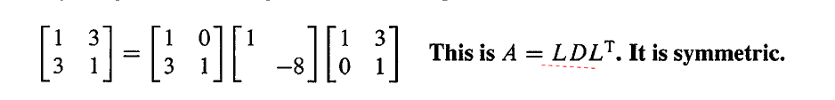
当 $L$L 变成 $I$I 的时候， $LD{L}^T$LDLT 就变成了 $ID{I}^T$IDIT，也就是由 $A$A 变成了 $D$D。 $A$A 的特征值为 4 和 -2， $D$D 的特征值为 1 和 -8。当 $L$L 中左下角的元素从 3 变到 0 的时候， $L$L 就变成了 $I$I。在这个过程中，如果特征值符号发生改变的话，那肯定会有一个中间时刻，这时候特征值为 0，也就意味着矩阵是奇异的。但是最后的矩阵 $D$D 一直有两个主元，始终是可逆的，从来不可能是奇异的，因此特征值的符号不会发生改变。

特别地，所有的特征值都大于零，也就是所有的主元都大于零，这种情况下，矩阵就称之为是正定的。

4. 重复的特征值

当没有重复特征值的时候，特征向量一定是线性不相关的，这时候矩阵一定可以被对角化。但是一个重复的特征值可能会导致特征向量的缺乏，这有些时候会发生在非对称矩阵上，但是对称矩阵一定会有足够的特征向量来进行对角化。

证明

获取更多精彩，请关注「seniusen」!