

目录
质数
试除法判定质数
根据定义 [ 1 , n ] [1, n] [1,n]中与 n n n互质的数的个数只有 1 1 1和他本身, 也就是约数个数为 0 0 0
, 因为约数是成对出现的, 只需要枚举较小的约数, 也就是 d ≤ n d d \le \frac{n}{d} d≤dn, 也就是 d 2 ≤ n d ^ 2 \le n d2≤n, 算法时间复杂度 O ( n ) O(\sqrt n) O(n)
#include <bits/stdc++.h>

using namespace std;

int n;

bool is_prime(int val) {

    if (val < 2) return false;
    for (int i = 2; i <= val / i; ++i) {

        if (val % i == 0) return false;
    }
    return true;
}

int main() {

    ios::sync_with_stdio(false);
    cin.tie(0);

    cin >> n;
    while (n--) {

        int val;
        cin >> val;
        cout << (is_prime(val) ? "Yes" : "No") << '\n';
    }

    return 0;
}
分解质因数
以为一个数的质因数只能从 2 2 2开始, 从小到大枚举所有的因子, 尝试 n n n的所有约数
算法时间复杂度 O ( n ) O(n) O(n)
引理: n n n中最多只包含一个大于 n \sqrt n n的质因子
证明: 假设存在两个大于 n \sqrt n n的质因子 p p p和 q q q, 因为 p p p和 q q q都是 n n n的质因子, 并且 p p p和 q q q互质, 因此 p × q p \times q p×q也是 n n n的质因子, 但是因为 p × q > n p \times q > n p×q>n, 因此矛盾, 证毕
大于 ( n ) \sqrt(n) (n)的质因子指数只能是 1 1 1, 因为如果指数 > 1 > 1 >1, 那么分解质因数的结果 > n > n >n, 矛盾
因此 n n n分解质因数后至多存在一个大于 n \sqrt n n的质因子, 并且指数是 1 1 1
优化后算法时间复杂度 O ( n ) O(\sqrt n) O(n)
#include <bits/stdc++.h>

using namespace std;

const int N = 110;

int n;

void solve() {

    int val;
    cin >> val;
    for (int i = 2; i <= val / i; ++i) {

        if (val % i == 0) {

            int cnt = 0;
            while (val % i == 0) {

                val /= i;
                cnt++;
            }
            if (cnt > 0) cout << i << ' ' << cnt << '\n';
        }
    }
    if (val > 1) cout << val << ' ' << 1 << '\n';
    cout << '\n';
}

int main() {

    ios::sync_with_stdio(false);
    cin.tie(0);

    cin >> n;
    while (n--) solve();

    return 0;
}
线性筛法求质数
算法时间复杂度 O ( n ) O(n) O(n)
#include <bits/stdc++.h>

using namespace std;

const int N = 1e6 + 10;

int n;
bool st[N];
int primes[N], cnt = 0;

void get_primes() {

    for (int i = 2; i <= n; ++i) {

        if (!st[i]) primes[cnt++] = i;
        for (int j = 0; i * primes[j] <= n; ++j) {

            st[i * primes[j]] = true;
            if (i % primes[j] == 0) break;
        }
    }
}

int main() {

    ios::sync_with_stdio(false);
    cin.tie(0);

    cin >> n;
    get_primes();

    cout << cnt << '\n';

    return 0;
}
关于线性筛法的证明
因为每个合数只会被它的最小质因子筛掉, 因此算法是正确的并且是线性的
为什么只会被最小质因子筛掉, 分情况进行讨论
- 情况 1 1 1, 因为第二维循环的质因子是从小到大枚举的, 当枚举到 i m o d p j = 0 i \mod p_j = 0 imodpj=0的时候, 说明 p j p_j pj是 i i i的最小质因子, 因此 p j p_j pj也是 i × p j i \times p_j i×pj的最小质因子, 因此将 i × p j i \times p_j i×pj筛掉
- 情况 2 2 2, 因为第二维循环的质因子是从小到大枚举的, 当没有枚举到 i m o d p j = 0 i \mod p_j = 0 imodpj=0的时候, p j p_j pj一定是 p j × i p_j \times i pj×i的最小质因子, 也需要筛掉
综上, 只要是从小到大枚举质因子, 就需要筛掉, 直到当前的 p j p_j pj已经是 i i i的最小质因子了, 退出循环, 保证算法的线性时间复杂度, 证毕
哥德巴赫猜想
要求输出 b − a b - a b−a最大的一组数据, 可以使用双指针算法, 但是会超时, 需要换一个算法
#include <bits/stdc++.h>

using namespace std;

const int N = 1e6 + 10;

int n;
int primes[N], cnt;
bool st[N];

void init() {

    for (int i = 2; i < N; ++i) {

        if (!st[i]) primes[cnt++] = i;
        for (int j = 0; i * primes[j] < N; ++j) {

            st[i * primes[j]] = true;
            if (i % primes[j] == 0) break;
        }
    }
}

void solve() {

    int i = 0, j = cnt - 1;

    bool flag = false;
    while (i <= j) {

        if (primes[i] + primes[j] == n) {

            printf("%d = %d + %d\n", n, primes[i], primes[j]);
            flag = true;
            break;
        }
        if (primes[i] + primes[j] < n) i++;
        else j--;
    }

    if (!flag) printf("Goldbach's conjecture is wrong.\n");
    return;
}

int main() {

    ios::sync_with_stdio(false);
    cin.tie(0);

    init();

    while (cin >> n, n) solve();

    return 0;
}
从小到大枚举所有的质数 a a a, 目标值是 n n n, 观察 n − a n - a n−a是否存在, 假设存在直接返回
#include <bits/stdc++.h>

using namespace std;

const int N = 1e6 + 10;

int n;
int primes[N], cnt;
bool st[N];

void init() {

    for (int i = 2; i < N; ++i) {

        if (!st[i]) primes[cnt++] = i;
        for (int j = 0; i * primes[j] < N; ++j) {

            st[i * primes[j]] = true;
            if (i % primes[j] == 0) break;
        }
    }
}

void solve() {

    for (int i = 1; i < cnt; ++i) {

        int val1 = primes[i];
        int val2 = n - val1;
        if (!st[val2]) {

            printf("%d = %d + %d\n", n, val1, val2);
            break;
        }
    }
}

int main() {

    ios::sync_with_stdio(false);
    cin.tie(0);

    init();

    while (cin >> n, n) solve();

    return 0;
}
CF776B
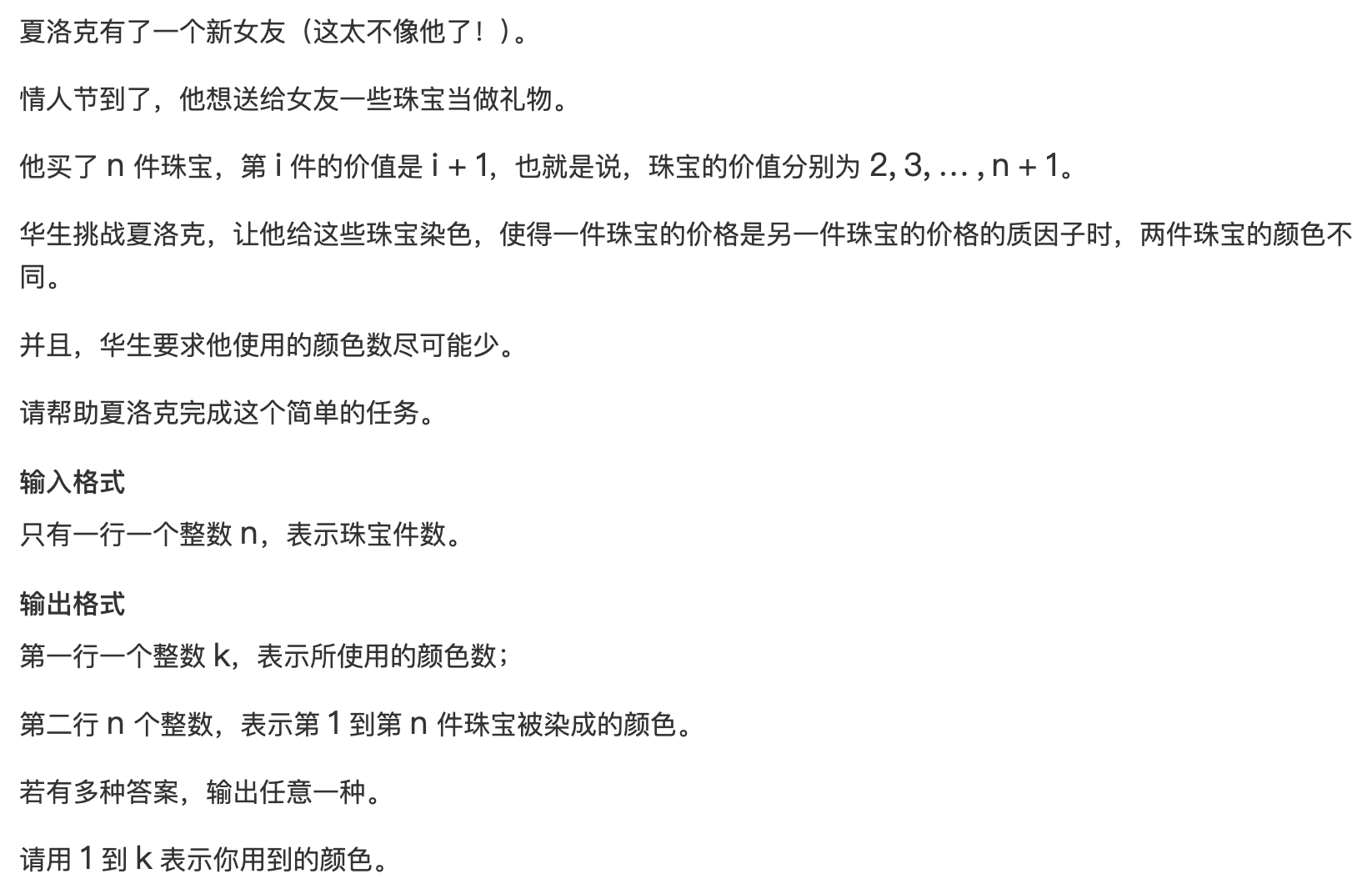
当珠子的数量 ≥ 3 \ge 3 ≥3, 发现只需要用两种颜色就能给珠子上色, 发现当前珠子是质数染色 1 1 1, 如果是合数染色 2 2 2
假设当前珠子数量 = = 2 ==2 ==2需要分类讨论
- 当前两个柱子都是质数, 使用 1 1 1个颜色
- 当前两个柱子都是合数, 使用 1 1 1个颜色
- 一个是质数, 另一个是合数, 并且该质数是合数的质因子, 需要两个颜色
- 一个是质数, 另一个是合数, 并且该质数不是该合数的质因子, 使用 1 1 1个颜色
假设当前珠子数量是 1 1 1
只需要使用 1 1 1个颜色
#include <bits/stdc++.h>

using namespace std;

const int N = 1e5 + 10;

int n, w[N];
int primes[N], cnt;
bool st[N];

void init() {

    for (int i = 2; i < N; ++i) {

        if (!st[i]) primes[cnt++] = i;
        for (int j = 0; i * primes[j] < N; ++j) {

            st[i * primes[j]] = true;
            if (i % primes[j] == 0) break;
        }
    }
}

int main() {

    ios::sync_with_stdio(false);
    cin.tie(0);

    init();

    cin >> n;
    for (int i = 0; i < n; ++i) w[i] = i + 2;

    if (n == 1) {

        cout << 1 << '\n' << 1 << '\n';
    }
    else if (n == 2) {

        int a = w[0], b = w[1];
        if (a > b) swap(a, b);
        if (b % a == 0) {

            cout << 2 << '\n';
            cout << 1 << ' ' << 2 << '\n';
        }
        else {

            cout << 1 << '\n';
            cout << 1 << ' ' << 1 << '\n';
        }
    }
    else {

        cout << 2 << '\n';
        for (int i = 0; i < n; ++i) {

            if (!st[w[i]]) cout << 1 << ' ';
            else cout << 2 << ' ';
        }
    }

    return 0;
}
质数距离
阶乘分解
约数
试除法求约数
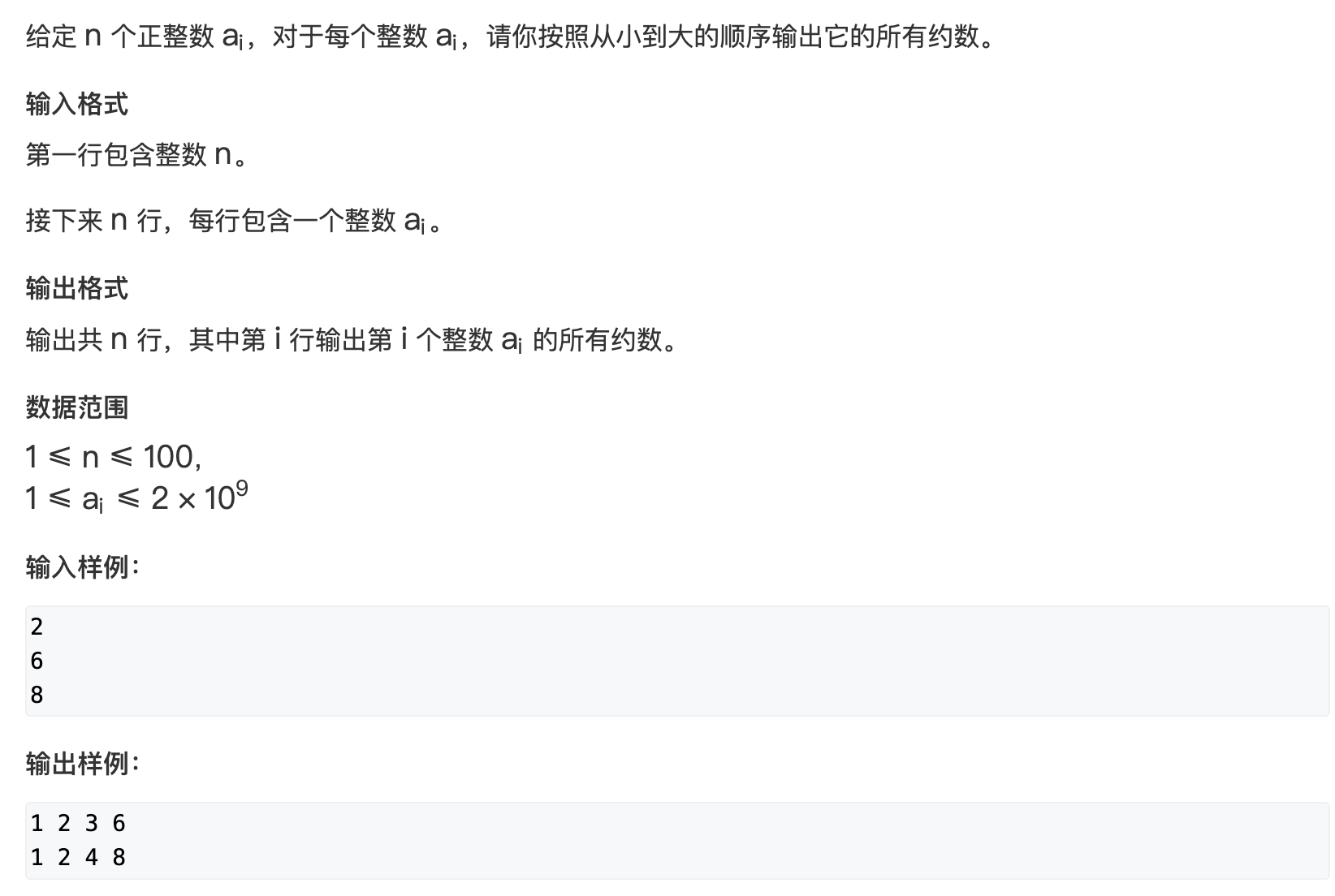
因为约数是成对出现的, 因此只需要枚举 d ≤ n d \le \sqrt n d≤n的情况, 并且大于 n \sqrt n n的约数只能是质数并且只能有一个, 计算约数后还需要排序去重
算法时间复杂度 O ( n + n log n ) O(\sqrt n + n\log n) O(n+nlogn)
#include <bits/stdc++.h>

using namespace std;

const int N = 110;

int n;

void solve() {

    int val;
    vector<int> nums;

    cin >> val;
    for (int i = 1; i <= val / i; ++i) {

        if (val % i == 0) {

            nums.push_back(i);
            if (val / i != i) nums.push_back(val / i);
        }
    }
    sort(nums.begin(), nums.end());
    for (int d : nums) cout << d << ' ';
    cout << '\n';
}

int main() {

    ios::sync_with_stdio(false);
    cin.tie(0);

    cin >> n;
    while (n--) solve();

    return 0;
}
约数个数
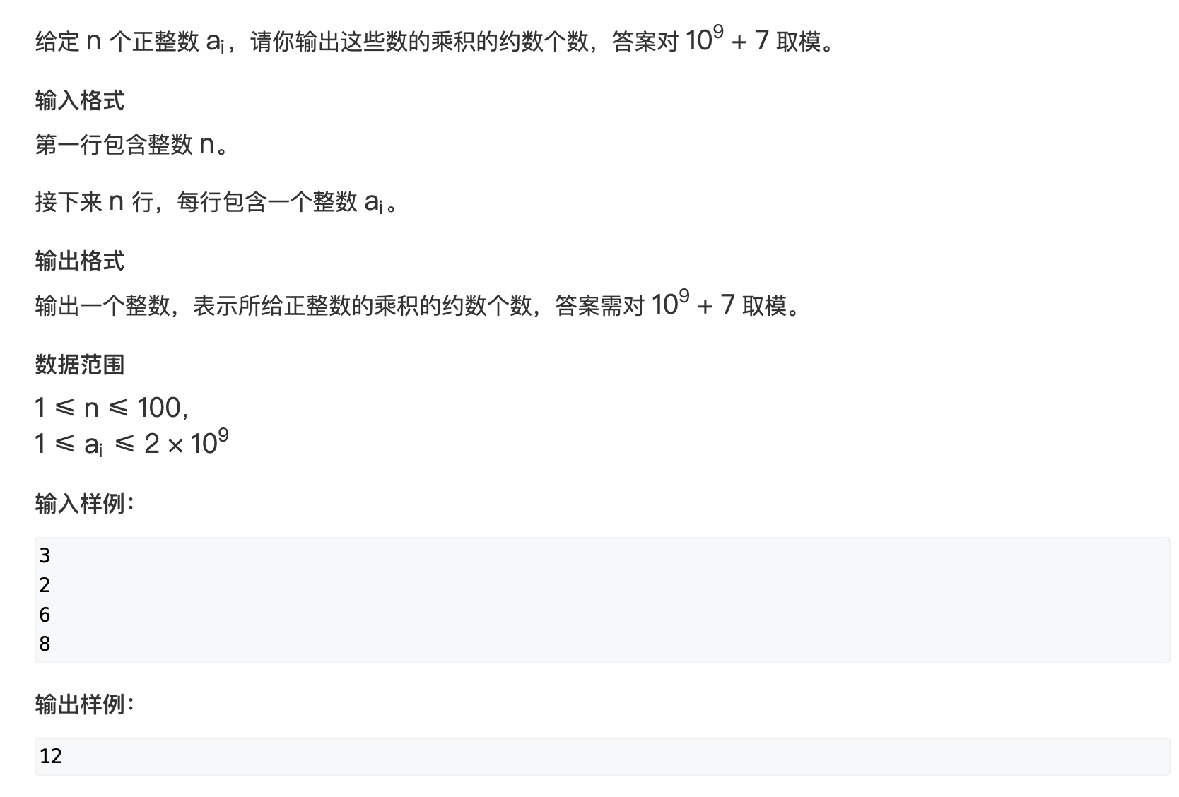
根据乘法原理, 约数个数 c n t = ( α 0 + 1 ) × ( α 1 + 1 ) × . . . × ( α k + 1 ) cnt = (\alpha _0 + 1) \times (\alpha _1 + 1) \times ... \times (\alpha _k + 1) cnt=(α0+1)×(α1+1)×...×(αk+1), 试除法分解质因数过程中求解指数的大小, 算法时间复杂度 O ( n ) O(\sqrt n) O(n)
#include <bits/stdc++.h>

using namespace std;

typedef long long LL;
const int MOD = 1e9 + 7;

int n;
unordered_map<int, int> mp;

void solve() {

    int val;
    cin >> val;
    for (int i = 2; i <= val / i; ++i) {

        while (val % i == 0) {

            val /= i;
            mp[i]++;
        }
    }
    if (val > 1) mp[val]++;
}

int main() {

    ios::sync_with_stdio(false);
    cin.tie(0);

    cin >> n;
    while (n--) solve();

    LL res = 1;
    for (auto [x, y] : mp) res = res * (y + 1) % MOD;

    cout << res << '\n';

    return 0;
}
约数之和
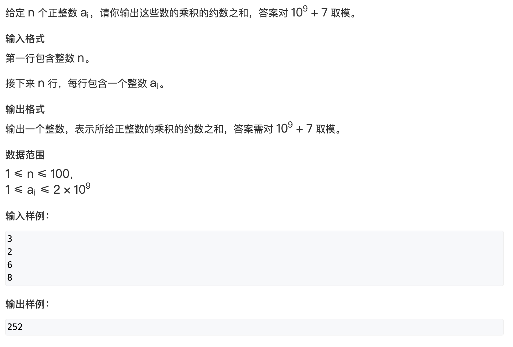
根据算术基本定理, 约数之和
s u m = ( p 1 0 + p 1 1 + . . . + p 1 α 1 ) ( p 2 0 + p 2 1 + . . . + p 2 α 2 ) . . . ( p k 0 + p k 1 + . . . + p k α k ) sum = (p _1 ^ 0 + p_1 ^ 1 + ... + p_1 ^ {\alpha_{1}})(p _2 ^ 0 + p_2 ^ 1 + ... + p_2 ^ {\alpha_{2}}) ... (p _k ^ 0 + p_k ^ 1 + ... + p_k ^ {\alpha_{k}}) sum=(p10+p11+...+p1α1)(p20+p21+...+p2α2)...(pk0+pk1+...+pkαk)
依旧是分解质因数, 计算结果要取模, 算法时间复杂度 O ( n ) O(\sqrt n) O(n)
注意在计算 t m p tmp tmp过程中要取模, 秦九韶算法求每一项, 内部的算法时间复杂度 O ( n ) O(n) O(n)
总的算法时间复杂度 O ( n n ) O(n \sqrt n) O(nn)
#include <bits/stdc++.h>

using namespace std;

typedef long long LL;
const int MOD = 1e9 + 7;

int n;
unordered_map<int, int> mp;

void solve() {

    int val;
    cin >> val;
    for (int i = 2; i <= val / i; ++i) {

        while (val % i == 0) {

            val /= i;
            mp[i]++;
        }
    }
    if (val > 1) mp[val]++;
}

int main() {

    ios::sync_with_stdio(false);
    cin.tie(0);

    cin >> n;
    while (n--) solve();

    LL res = 1;
    for (auto [x, y] : mp) {

        if (x != 0) {

            LL tmp = 1;
            // 秦九韶算法求p ^ 0 + p ^ 1 + ... + p ^ n
            while (y--) tmp = (tmp * x + 1) % MOD;
            res = res * tmp % MOD;
        }
    }

    cout << res << '\n';

    return 0;
}
求最大公约数-欧几里得算法的证明和实现
轻拍牛头
樱花
反素数
Hankson的趣味题
Euler函数
容斥原理证明欧拉函数
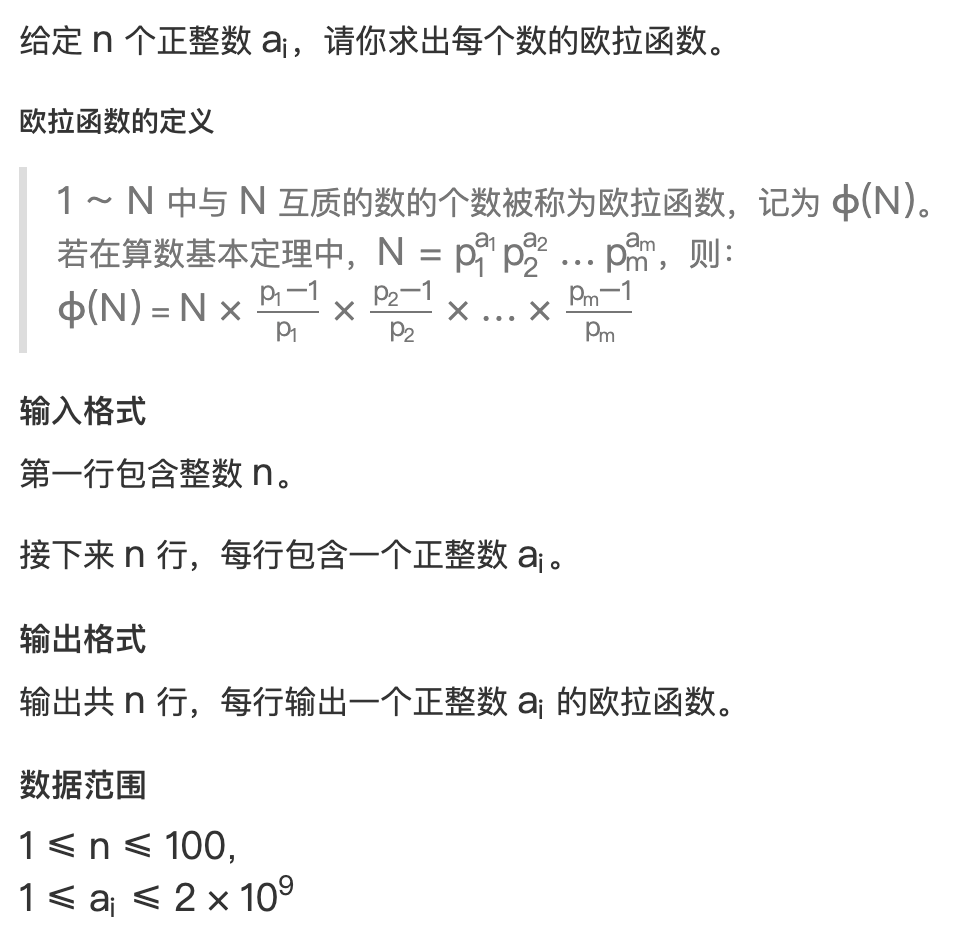
将 n n n分解质因数, 算法时间复杂度 O ( n ) O(\sqrt n) O(n), 一个数的质因子最大数量是 log n \log n logn, 因此求一个数字的欧拉函数算法时间复杂度 O ( log m × m ) O(\log m \times \sqrt m) O(logm×m), 一共有 n n n个数字, 算法时间复杂度 O ( O ( n × log m × m ) ) O(O(n \times \log m \times \sqrt m)) O(O(n×logm×m))
注意为了避免超出 i n t int int范围, 先做除法再做乘法
#include <bits/stdc++.h>

using namespace std;

int n;

int solve() {

    int val;
    cin >> val;
    double res = val;
    for (int i = 2; i <= val / i; ++i) {

        if (val % i == 0) {

            res = res / i * (i - 1);
            while (val % i == 0) val /= i;
        }
    }
    if (val > 1) res = res / val * (val - 1);
    return res;
}

int main() {

    ios::sync_with_stdio(false);
    cin.tie(0), cout.tie(0);

    cin >> n;
    while (n--) {

        int res = solve();
        cout << res << '\n';
    }

    return 0;
}
线性筛法求欧拉函数
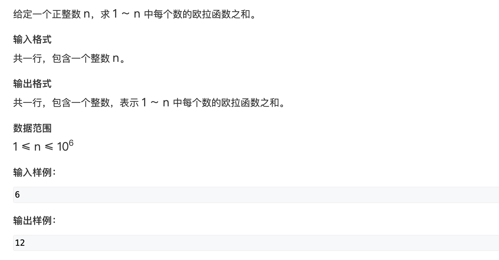
在线性筛质数基础上, 计算欧拉函数, 算法时间复杂度 O ( n ) O(n) O(n)
下面是如何在筛质数途中计算 E u l e r ( i ) Euler(i) Euler(i)
如果当前数字是质数 i i i, 那么 ϕ ( i ) = p − 1 \phi(i) = p - 1 ϕ(i)=p−1
如果当前数字 p p p是 i i i的最小质因子, ϕ ( i ) = i × k × p − 1 p \phi (i) = i \times k \times \frac{p - 1}{p} ϕ(i)=i×k×pp−1, 因此 ϕ ( i × j ) = p × ϕ ( i ) \phi (i \times j) = p \times \phi (i) ϕ(i×j)=p×ϕ(i)
如果当前数字 p p p比 i i i的最小质因子小, 那么 p p p是 i × p i \times p i×p的最小质因子, 那么 ϕ ( i × j ) = ϕ ( i ) × p × p − 1 p \phi (i \times j) = \phi (i) \times p \times \frac{p - 1}{p} ϕ(i×j)=ϕ(i)×p×pp−1
#include <bits/stdc++.h>

using namespace std;

typedef long long LL;
const int N = 1e6 + 10;

int n;
bool st[N];
int primes[N], phi[N], cnt;

void init() {

    phi[1] = 1;
    for (int i = 2; i <= n; ++i) {

        if (!st[i]) {

            phi[i] = i - 1;
            primes[cnt++] = i;
        }
        for (int j = 0; primes[j] <= n / i; ++j) {

            st[i * primes[j]] = true;
            if (i % primes[j] == 0) {

                phi[i * primes[j]] = primes[j] * phi[i];
                break;
            }
            else phi[i * primes[j]] = phi[i] * (primes[j] - 1);
        }
    }
}

int main() {

    ios::sync_with_stdio(false);
    cin.tie(0), cout.tie(0);

    cin >> n;
    init();

    LL res = 0;
    for (int i = 1; i <= n; ++i) res += (LL) phi[i];

    cout << res << '\n';
    return 0;
}
可见的点
最大公约数
快速幂, 龟速乘
快速幂算法
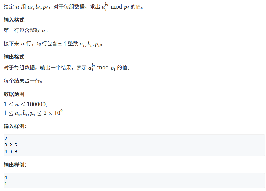
快速幂算法核心是反复平方法, 假设计算 a b m o d M a ^ b \mod M abmodM, 可以预处理 a 2 0 , a 2 1 , a 2 2 , . . . a ^ {2 ^ 0}, a ^ {2 ^ 1}, a ^ {2 ^ 2}, ... a20,a21,a22,... , 然后将 b b b展开为二进制数, 有 1 1 1的地方说明要参与运算, 算法时间复杂度 O ( log b ) O(\log b) O(logb)
#include <bits/stdc++.h>

using namespace std;

typedef long long LL;

int pow(int a, int b, int p) {

    a = a % p;
    int res = 1;

    while (b) {

        if (b & 1) res = (LL) res * a % p;
        a = (LL) a * a % p;
        b >>= 1;
    }
    return res % p;
}

int main() {

    ios::sync_with_stdio(false);
    cin.tie(0), cout.tie(0);

    int n;
    cin >> n;
    while (n--) {

        int a, b, p;
        cin >> a >> b >> p;
        cout << pow(a, b, p) << '\n';
    }

    return 0;
}
快速幂求逆元
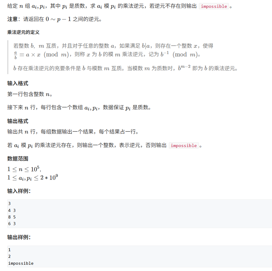
乘法逆元的意思就是 a b ≡ a × x ( m o d n ) \frac {a}{b} \equiv a \times x (\mod n) ba≡a×x(modn), x x x就是乘法逆元, 也就是在 m o d n \mod n modn的情况下, 可以将除法转化为乘法
欧拉定理: a ϕ ( n ) ≡ 1 ( m o d n ) a ^ {\phi (n)} \equiv 1 (\mod n) aϕ(n)≡1(modn), 其中 a a a与 n n n互质
欧拉定理的证明: 对于数字 n n n的质因子如下 a 1 , a 2 , a 3 , . . . , a ϕ ( n ) a_1, a_2, a_3, ..., a_{\phi(n)} a1,a2,a3,...,aϕ(n), 一共 ϕ ( n ) \phi(n) ϕ(n)个, 那么因为 a a a与 n n n会互质, 因此 a ⋅ a 1 , a ⋅ a 2 , . . . , a ⋅ a ϕ ( n ) a\cdot a_1, a \cdot a_2, ... , a\cdot a_{\phi(n)} a⋅a1,a⋅a2,...,a⋅aϕ(n)也与 n n n互质, 但是因为 1 1 1到 n n n中与 n n n互质的数的是确定的, 两段其实是一个集合, 也就是有 a 1 × a 2 × . . . × a ϕ ( n ) = a ⋅ a 1 × a ⋅ a 2 × . . . × a ⋅ a ϕ ( n ) a_1 \times a_2 \times... \times a_{\phi(n)} = a\cdot a_1 \times a \cdot a_2\times ... \times a\cdot a_{\phi(n)} a1×a2×...×aϕ(n)=a⋅a1×a⋅a2×...×a⋅aϕ(n)
也就是等于 a ϕ ( n ) × k = k a ^ {\phi(n)}\times k = k aϕ(n)×k=k, k = a 1 × a 2 × . . . × a ϕ ( n ) k = a_1 \times a_2 \times... \times a_{\phi(n)} k=a1×a2×...×aϕ(n), 因为每一个质因子都与 n n n互质, 乘起来也与 n n n互质, 因此有 a ϕ ( n ) ≡ 1 ( m o d n ) a ^ {\phi (n)} \equiv 1 (\mod n) aϕ(n)≡1(modn), 证毕
费马小定理: a p − 1 ≡ 1 ( m o d p ) a ^ {p - 1} \equiv 1 (\mod p) ap−1≡1(modp)
根据费马小定理, 计算乘法逆元的过程可以表示为 a ⋅ a p − 2 ≡ 1 ( m o d n ) a\cdot a ^ {p - 2} \equiv 1 (\mod n) a⋅ap−2≡1(modn), a p − 2 a ^ {p - 2} ap−2就是 a a a在 m o d p \mod p modp下的乘法逆元, 其中 a a a与 n n n互质
利用快速幂计算 a p − 2 a ^ {p - 2} ap−2, 时间复杂度 O ( log b ) O(\log b) O(logb)
#include <bits/stdc++.h>

using namespace std;

typedef long long LL;

LL pow(int a, int b, int p) {

    LL res = 1 % p;
    a %= p;
    b %= p;
    while (b) {

        if (b & 1) res = (LL) res * a % p;
        b >>= 1;
        a = (LL) a * a % p;
    }
    return res;
}

int main() {

    ios::sync_with_stdio(false);
    cin.tie(0);

    int n;
    cin >> n;
    while (n--) {

        int a, p;
        cin >> a >> p;
        if (a % p == 0) {

            cout << "impossible" << '\n';
            continue;
        }
        LL res = pow(a, p - 2, p);
        cout << res << '\n';
    }

    return 0;
}
龟速乘算法
将 b b b拆分为二进制数, 预处理
a × 2 0 , a × 2 1 , a × 2 2 , a × 2 3 , … a \times 2^0, a \times 2^1, a \times 2^2, a \times 2^3, \ldots a×20,a×21,a×22,a×23,…
然后利用二进制拼凑的思想, 凑出 b b b
正常的计算乘法时间复杂度是 O ( 1 ) O(1) O(1), 但是该算法的时间复杂度是 O ( log b ) O(\log b) O(logb)
#include <bits/stdc++.h>

using namespace std;

typedef long long LL;

LL slow_mul(LL a, LL b, LL p) {

    LL res = 0;
    while (b) {

        if (b & 1) res = (res + a) % p;
        b >>= 1;
        a = (a + a) % p;
    }
    return res;
}

int main() {

    ios::sync_with_stdio(false);
    cin.tie(0);

    LL a, b, p;
    cin >> a >> b >> p;

    cout << slow_mul(a, b, p) << '\n';
    return 0;
}
序列的第K个数
越狱
同余
同余方程
青蛙的约会
最幸运的数字
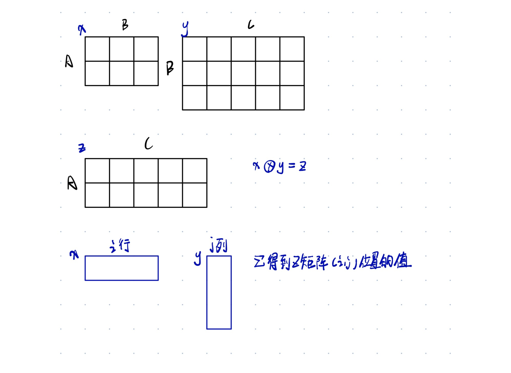
矩阵乘法
Fibonacci数列
佳佳的斐波那契
GT考试
扩展欧几里得算法

裴蜀定理: 存在整数 x x x, y y y, 使得 a x + b y = gcd ( a , b ) ax + by = \gcd (a, b) ax+by=gcd(a,b)
目标就是求 x x x和 y y y, 计算得到是一组特解, 原方程的通解等于特解 + 线性其次解
算法流程: 当计算到 b = 0 b = 0 b=0的时候, gcd ( a , b ) = a \gcd (a, b) = a gcd(a,b)=a, 那么得到特殊解 x = 1 x = 1 x=1, y = 0 y = 0 y=0
否则, g c d ( a , b ) = d = a x + b y gcd(a, b) = d = ax + by gcd(a,b)=d=ax+by
由欧几里得算法可知 gcd ( a , b ) = gcd ( b , a m o d b ) \gcd(a, b) = \gcd(b, a \mod b) gcd(a,b)=gcd(b,amodb)
那么有 gcd ( b , a m o d b ) = a x + b y \gcd(b, a \mod b) = ax + by gcd(b,amodb)=ax+by
展开得到 b x ′ + ( a − b ⋅ ⌊ a b ⌋ ) ⋅ y ′ = d bx' + (a - b\cdot {\left \lfloor \frac{a}{b} \right \rfloor }) \cdot y' = d bx′+(a−b⋅⌊ba⌋)⋅y′=d
整理得到 a y ′ + b ⋅ ( x ′ − ⌊ a b ⌋ ⋅ y ′ ) = d ay' + b\cdot (x' - \left \lfloor \frac{a}{b} \right \rfloor \cdot y') = d ay′+b⋅(x′−⌊ba⌋⋅y′)=d
那么在计算过程中递归的将 x x x赋值为 y y y, 将 y y y赋值为 x ′ − ⌊ a b ⌋ ⋅ y ′ x' - \left \lfloor \frac{a}{b} \right \rfloor \cdot y' x′−⌊ba⌋⋅y′
得到特殊解 ( x 0 , y 0 ) (x_0, y_0) (x0,y0)
对于得到了通解的方程 a x 0 + b y 0 = d ax_0 + by_0 = d ax0+by0=d, 等价转化为
a ( x 0 + b d ) + b ( y 0 − a d ) = d a(x_0 + \frac{b}{d}) + b(y_0 - \frac{a}{d}) = d a(x0+db)+b(y0−da)=d
通解可以表示为 x = x 0 + b d ⋅ k x = x_0 + \frac{b}{d} \cdot k x=x0+db⋅k, y = y 0 + a d ⋅ k y = y_0 + \frac{a}{d} \cdot k y=y0+da⋅k, k ∈ Z k \in Z k∈Z
观察推导过程, 当前状态 a x + b y ax + by ax+by是由上一个状态 gcd ( a , b ) \gcd (a, b) gcd(a,b)的 x ′ , y ′ x', y' x′,y′推导过来的, 因此可以在函数返回过程中, 利用上一级递归的结果计算当前层的 x x x和 y y y
#include <bits/stdc++.h>

using namespace std;

int exgcd(int a, int b, int &x, int &y) {

    if (b == 0) {

        x = 1, y = 0;
        return a;
    }

    int _x, _y;
    int d = exgcd(b, a % b, _x, _y);
    x = _y, y = _x - (a / b) * _y;
    return d;
}

int main() {

    ios::sync_with_stdio(false);
    cin.tie(0), cout.tie(0);

    int n;
    cin >> n;
    while (n--) {

        int a, b, x, y;
        cin >> a >> b;
        exgcd(a, b, x, y);
        cout << x << ' ' << y << '\n';
    }

    return 0;
}
线性同余方程
扩展欧几里得算法的简单应用
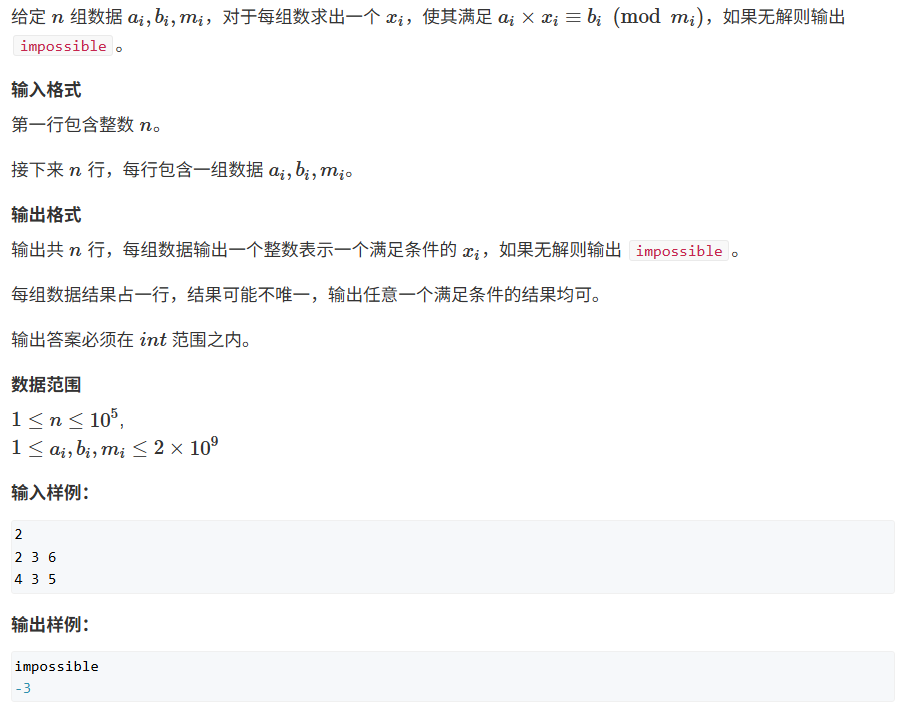
将方程转化 m i × y i + b i = a i × x i m_i \times y_i + b_i = a_i \times x_i mi×yi+bi=ai×xi
继续变形 a i × x i + m i × y i = b i a_i \times x_i + m_i \times y_i = b_i ai×xi+mi×yi=bi, 其中 y i ∈ Z y_i \in Z yi∈Z
能使用扩展欧几里得算法求解线性同余方程的前提条件是 gcd ( a i , m i ) ∣ b i \gcd(a_i, m_i) | b_i gcd(ai,mi)∣bi, 假设 k ⋅ gcd ( a , b ) = b i k \cdot \gcd(a, b) = b_i k⋅gcd(a,b)=bi, 并且计算拓展欧几里得算法得到的通解是 ( x 0 , y 0 ) (x_0, y_0) (x0,y0), 那么实际方程的解是 ( k ⋅ x 0 , k ⋅ y 0 ) (k \cdot x_0, k \cdot y_0) (k⋅x0,k⋅y0)
#include <bits/stdc++.h>

using namespace std;

typedef long long LL;

int n;
int a, b, m;

int exgcd(int a, int b, int &x, int &y) {

    if (b == 0) {

        x = 1, y = 0;
        return a;
    }

    int _x, _y;
    int d = exgcd(b, a % b, _x, _y);
    x = _y, y = _x - (a / b) * _y;
    return d;
}

int main() {

    ios::sync_with_stdio(false);
    cin.tie(0), cout.tie(0);

    cin >> n;
    while (n--) {

        cin >> a >> b >> m;
        int x, y;
        int d = exgcd(a, m, x, y);
        if (b % d) {

            cout << "impossible" << '\n';
            continue;
        }
        cout << (LL) x * (b / d) % m << '\n';
    }

    return 0;
}
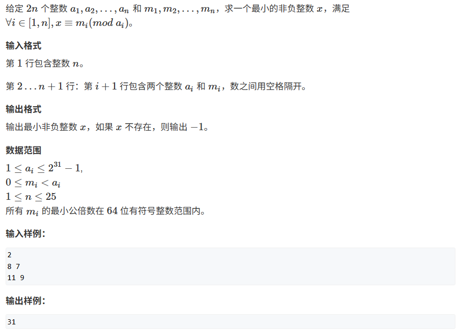
中国剩余定理
m m m之间两两互质, 线性同余方程组
{ x ≡ r 1 ( m o d m 1 ) x ≡ r 2 ( m o d m 2 ) x ≡ r 3 ( m o d m 3 ) ⋮ x ≡ r n ( m o d m n ) \left\{\begin{array}{l} x \equiv r_{1}\left(\bmod m_{1}\right) \\ x \equiv r_{2}\left(\bmod m_{2}\right) \\ x \equiv r_{3}\left(\bmod m_{3}\right) \\ \vdots \\ x \equiv r_{n}\left(\bmod m_{n}\right) \end{array}\right. ⎩ ⎨ ⎧x≡r1(modm1)x≡r2(modm2)x≡r3(modm3)⋮x≡rn(modmn)
有公式解, M = m 1 ⋅ m 2 ⋅ . . . ⋅ m k M = m_1 \cdot m_2 \cdot ... \cdot m_k M=m1⋅m2⋅...⋅mk, M i = M m i M_i = \frac {M}{m_i} Mi=miM, M i M_i Mi是除了 m i m_i mi之外其他所有 m m m的乘积
因为 m m m之间两两互质, M i M_i Mi和 m i m_i mi之间互质, 因此可以求出 M i − 1 M_i ^ {-1} Mi−1, 也就是 M i M_i Mi m o d m i \mod m_i modmi的逆
通解 x = r 1 × M 1 × M 1 − 1 + r 2 × M 2 × M 2 − 1 + . . . + r n × M n × M n − 1 x = r_1 \times M_1 \times M_1 ^ {-1} + r_2 \times M_2 \times M_2 ^ {-1} + ... +r_n \times M_n \times M_n ^ {-1} x=r1×M1×M1−1+r2×M2×M2−1+...+rn×Mn×Mn−1
M 1 x ≡ 1 ( m o d m ) M_1x \equiv 1 (\mod m) M1x≡1(modm), x x x就是逆元, 但是因为 m m m不一定是质数, 不能用快速幂求逆的方式(费马小定理), 只能使用扩展欧几里得算法求逆
为什么 x x x是通解?
观察通解方程, 假设在 m o d m k \mod m_k modmk的情况下, 因为 M k × M k − 1 M_k \times M_k ^ {-1} Mk×Mk−1在 m o d m k \mod m_k modmk的情况下等于 1 1 1, 因此 r k × M k × M k − 1 = 1 r_k \times M_k \times M_k ^ {-1} = 1 rk×Mk×Mk−1=1, 观察其他项 r m × M m × M m − 1 r_m \times M_m \times M_m ^ {-1} rm×Mm×Mm−1, 因为 M m M_m Mm包含了 m k m_k mk, 也就是 m k m_k mk的倍数, 在 m o d m k \mod m_k modmk的情况下就是 0 0 0, 也就是 r m × 0 × M m − 1 r_m \times 0 \times M_m ^ {-1} rm×0×Mm−1, 因此通解在 m o d m k \mod m_k modmk的情况下, 结果就变成了 x = r k x = r_k x=rk, 因此 x x x是上述同余方程的通解
表达整数的奇怪方式
注意到因为给定的 m m m之间不互质, 因此不能直接使用中国剩余定理解决
{ x ≡ m 1 ( m o d a 1 ) x ≡ m 2 ( m o d a 2 ) x ≡ m 3 ( m o d a 3 ) ⋮ x ≡ m n ( m o d a n ) \left\{\begin{array}{l} x \equiv m_{1}\left(\bmod a_{1}\right) \\ x \equiv m_{2}\left(\bmod a_{2}\right) \\ x \equiv m_{3}\left(\bmod a_{3}\right) \\ \vdots \\ x \equiv m_{n}\left(\bmod a_{n}\right) \end{array}\right. ⎩ ⎨ ⎧x≡m1(moda1)x≡m2(moda2)x≡m3(moda3)⋮x≡mn(modan)
将上述等式变形, 得到
{ k 1 a 1 + m 1 = x k 2 a 2 + m 2 = x k 3 a 3 + m 3 = x ⋮ k n a n + m n = x \left\{\begin{array}{l} k_1a_1 + m_1 = x \\ k_2a_2 + m_2 = x \\ k_3a_3 + m_3 = x \\ \vdots \\ k_na_n + m_n = x \end{array}\right. ⎩ ⎨ ⎧k1a1+m1=xk2a2+m2=xk3a3+m3=x⋮knan+mn=x
先将问题简化, 取出前两个式子, 得到 k 1 a 1 + m 1 = k 2 a 2 + m 2 k_1a_1 + m_1 = k_2a_2 + m_2 k1a1+m1=k2a2+m2
继续化简
k 1 a 1 − k 2 a 2 = m 2 − m 1 k_1a_1 - k_2a_2 = m_2 - m_1 k1a1−k2a2=m2−m1
可以使用扩展欧几里得算法求解的前提条件(也就是有解的前提条件)是 gcd ( a 1 , a 2 ) ∣ m 2 − m 1 \gcd(a_1, a_2) | m_2 - m_1 gcd(a1,a2)∣m2−m1
假设求出了 ( k 1 ′ , k 2 ′ ) (k_1 ', k_2 ') (k1′,k2′), 根据扩展欧几里得算法, 得到通解
{ k 1 = k 1 ′ + k ⋅ a 2 d k 2 = k 2 ′ − k ⋅ a 1 d \left\{\begin{array}{l} k1 = k1' + k \cdot \frac{a_2}{d} \\ k2 = k2' - k \cdot \frac{a_1}{d} \\ \end{array}\right. { k1=k1′+k⋅da2k2=k2′−k⋅da1
那么 x = ( k 1 ′ + k ⋅ a 2 d ) a 1 + m 1 x = ( k1' + k \cdot \frac{a_2}{d}) a_1 + m_1 x=(k1′+k⋅da2)a1+m1, 就是 x x x的所有解
x = a 1 k 1 ′ + m 1 + k ⋅ a 1 a 2 d x = a_1k_1' + m_1 + k \cdot \frac{a_1a_2}{d} x=a1k1′+m1+k⋅da1a2, 其中 a 1 a 2 d \frac{a_1a_2}{d} da1a2是最小公倍数 [ a 1 , a 2 ] [a_1, a_2] [a1,a2]
也就是 x = a 1 k 1 ′ + m 1 + k ⋅ [ a 1 , a 2 ] x = a_1k_1' + m_1 + k \cdot [a_1, a_2] x=a1k1′+m1+k⋅[a1,a2], 前面的 a 1 k 1 ′ + m 1 a_1k_1' + m_1 a1k1′+m1 是定值, k ⋅ [ a 1 , a 2 ] k \cdot [a_1, a_2] k⋅[a1,a2]可以记作新的 k ′ a ′ k'a' k′a′
这样就将两个式子合并成了一个式子 k ′ a ′ + m ′ = x k'a' + m' = x k′a′+m′=x
一共 n n n个方程合并 n − 1 n - 1 n−1次, 最终合并为一个方程 x = k a + m x = ka + m x=ka+m, 希望计算 x x x的最小正整数解, x ≡ m ( m o d a ) x \equiv m (\mod a) x≡m(moda)
关于如何计算 x x x的最小正整数解, 可以分情况讨论, 当 m ≥ 0 m \ge 0 m≥0,
int min_x = m % a, 当 m < 0 m < 0 m<0,int min_x = (m % a + a) % a, 综上可以使用一个方法计算得到int min_x = (m % a + a) % m
注意将 a 1 , a 2 , m 1 , m 2 a_1, a_2, m_1, m_2 a1,a2,m1,m2的数据类型转化为
long long否则会产生溢出风险
#include <bits/stdc++.h>

using namespace std;

typedef long long LL;

int n;
LL a1, a2, m1, m2;

LL exgcd(LL a, LL b, LL &x, LL &y) {

    if (b == 0) {

        x = 1, y = 0;
        return a;
    }

    LL _x, _y;
    LL d = exgcd(b, a % b, _x, _y);
    x = _y, y = _x - (a / b) * _y;
    return d;
}

int main() {

    ios::sync_with_stdio(false);
    cin.tie(0);

    cin >> n;
    cin >> a1 >> m1;
    n--;

    LL k1 = 1, k2 = 1;
    while (n--) {

        cin >> a2 >> m2;
        LL d = exgcd(a1, a2, k1, k2);
        if (abs(m2 - m1) % d) {

            k1 = -1;
            break;
        }
        // 因为通解的表达方式是k * (a2 / gcd), 其实是对(a2 / gcd)取模
        LL mod = a2 / d;
        k1 = (LL) k1 * (m2 - m1) / d;

        // 计算K1的最小正整数解
        k1 = (k1 % mod + mod) % mod;
        m1 = (LL) a1 * k1 + m1;
        a1 = a1 / d * a2;
    }

    if (k1 == -1) cout << k1 << '\n';
    else {

        LL res = (m1 % a1 + a1) % a1;
        cout << res << '\n';
    }

    return 0;
}
曹冲养猪
高斯消元
高斯消元解线性方程组
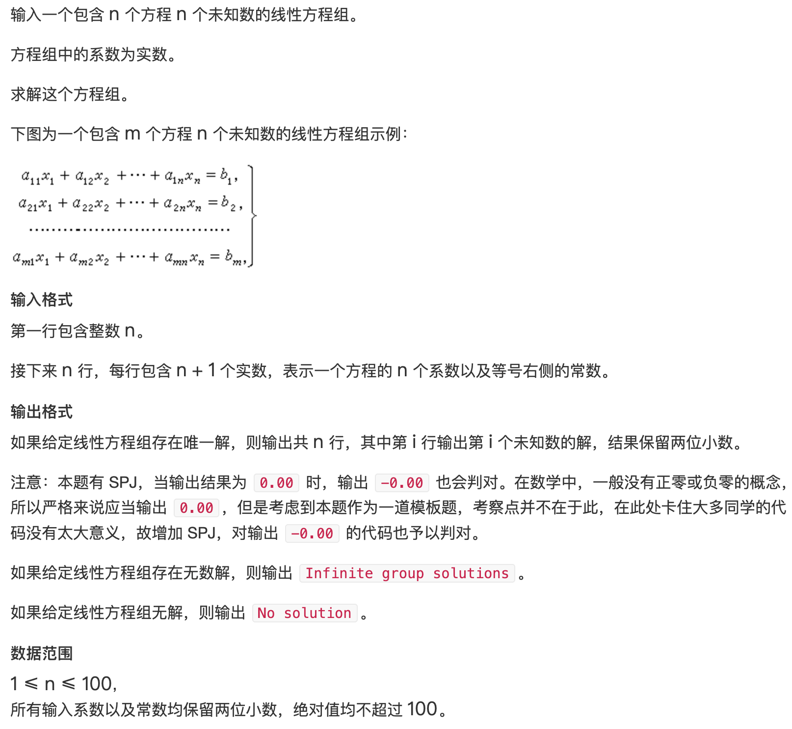
算法时间复杂度一般为 O ( n 3 ) O(n ^ 3) O(n3), 求解多元线性方程组
a 11 x 1 + a 12 x 2 + ⋯ + a 1 n x n = b 1 a 21 x 1 + a 22 x 2 + ⋯ + a 2 n x n = b 2 … … … … … … … … … … … a m 1 x 1 + a m 2 x 2 + ⋯ + a m n x n = b m } \left.\begin{array}{r} a_{11} x_{1}+a_{12} x_{2}+\cdots+a_{1 n} x_{n}=b_{1} \\ a_{21} x_{1}+a_{22} x_{2}+\cdots+a_{2 n} x_{n}=b_{2} \\ \ldots \ldots \ldots \ldots \ldots \ldots \ldots \ldots \ldots \ldots \ldots \\ a_{m 1} x_{1}+a_{m 2} x_{2}+\cdots+a_{m n} x_{n}=b_{m} \end{array}\right\} a11x1+a12x2+⋯+a1nxn=b1a21x1+a22x2+⋯+a2nxn=b2……………………………am1x1+am2x2+⋯+amnxn=bm⎭ ⎬ ⎫
会输入一个 n × ( n + 1 ) n \times (n + 1) n×(n+1)的系数矩阵
解的情况有三种, 无解, 无穷多组解, 唯一解
对系数矩阵进行初等行列变换, 转化成最简阶梯型矩阵
- 某一行乘一个非零的数
- 交换某两行
- 把某行的若干倍加到另一行上去
保证不会影响方程组的解的情况
- 完美阶梯型有唯一组解
- 左边没有未知数, 右边是非零的情况, 说明无解
- 经过变换后得到的不是完美阶梯型, 出现了 0 = 0 0 = 0 0=0的情况, 说明有无穷多组解
高斯消元的过程, 首先枚举每一列 c c c
- 在所有行中找到当前列绝对值最大的数的那一行
- 将该行交换到第一行
- 将当前列 c c c的数字变为 1 1 1
- 用当前行消除剩余行使得剩余行的当前列 c c c的值为 0 0 0
如果最终结果是 n n n个方程 n n n个未知数, 那就是唯一解的, 从最后一个方程上推, 也就是得到对角矩阵
#include <bits/stdc++.h>

using namespace std;

const int N = 110;
const double EPS = 1e-10;

int n;
double f[N][N];

int gauss() {

    int r, c;
    for (r = c = 0; c < n; ++c) {

        int t = r;
        for (int i = r + 1; i < n; ++i) {

            if (fabs(f[i][c]) > fabs(f[t][c])) t = i;
        }
        if (fabs(f[t][c]) < EPS) continue;
        for (int i = c; i < n + 1; ++i) swap(f[r][i], f[t][i]);
        for (int i = n; i >= c; --i) f[r][i] /= f[r][c];
        for (int i = r + 1; i < n; ++i) {

            if (fabs(f[i][c]) < EPS) continue;
            for (int j = n; j >= c; --j) {

                f[i][j] -= f[r][j] * f[i][c];
            }
        }
        r++;
    }

    if (r < n) {

        for (int i = r; i < n; ++i) {

            if (fabs(f[i][n])) return 2;
        }
        return 1;
    }

    for (int i = n - 1; i >= 0; --i) {

        for (int j = i + 1; j < n; ++j) {

            f[i][n] -= f[i][j] * f[j][n];
        }
    }

    return 0;
}


int main() {

    ios::sync_with_stdio(false);
    cin.tie(0), cout.tie(0);

    cin >> n;
    for (int i = 0; i < n; ++i) {

        for (int j = 0; j < n + 1; ++j) {

            cin >> f[i][j];
        }
    }

    int res = gauss();
    if (res == 2) cout << "No solution" << '\n';
    else if (res == 1) cout << "Infinite group solutions" << '\n';
    else {

        for (int i = 0; i < n; ++i) printf("%.2lf\n", f[i][n]);
    }

    return 0;
}
球形空间产生器
高斯消元解异或线性方程组
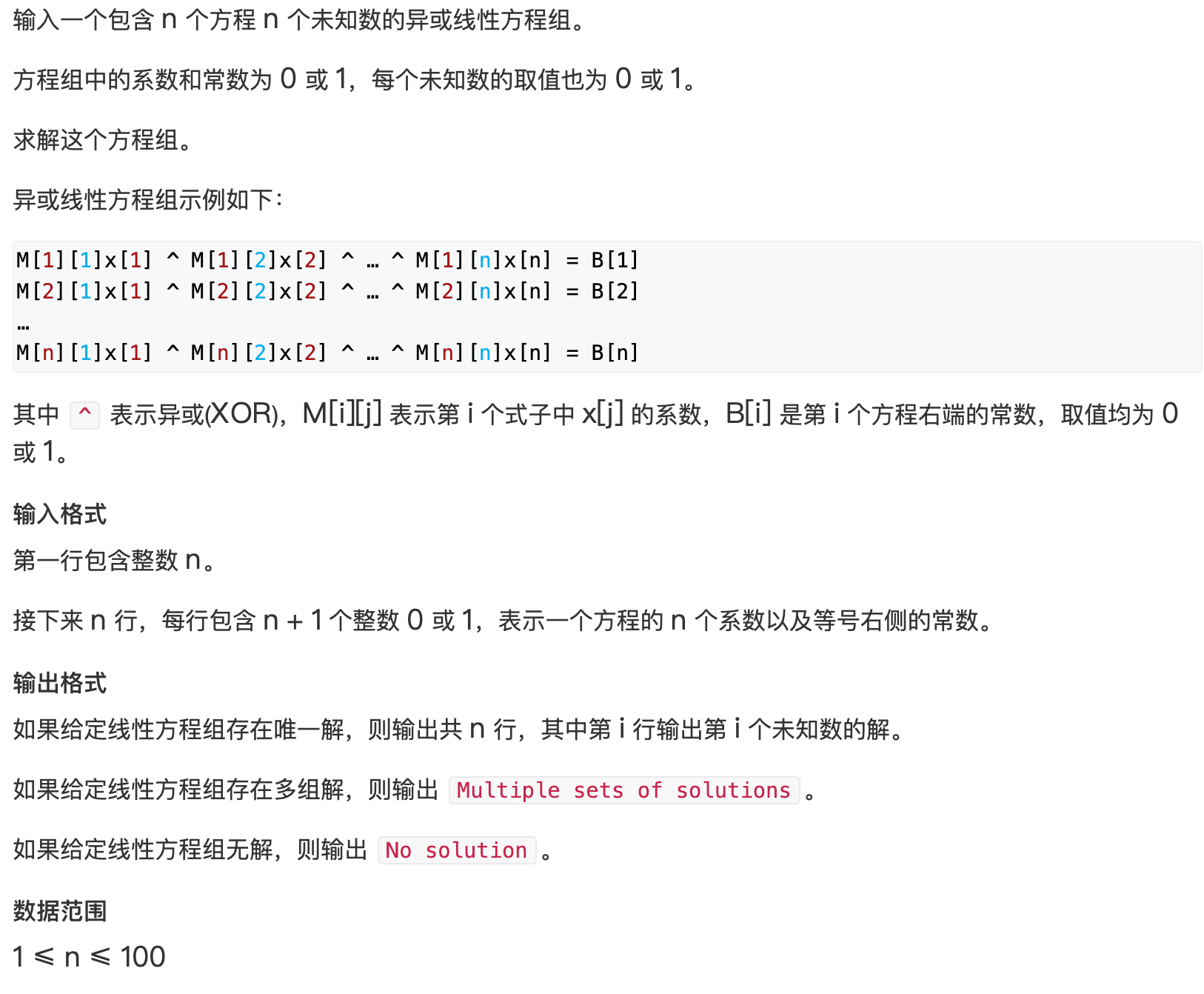
与高斯消元解线性方程组类似, 算法时间复杂度 O ( n 3 ) O(n ^ 3) O(n3)
#include <bits/stdc++.h>

using namespace std;

const int N = 110;

int n, f[N][N];

int gauss() {

    int r, c;
    for (r = c = 0; c < n; ++c) {

        int t = r;
        for (int i = r + 1; i < n; ++i) {

            if (f[i][c]) {

                t = i;
                break;
            }
        }
        if (!f[t][c]) continue;
        for (int i = c; i < n + 1; ++i) swap(f[r][i], f[t][i]);
        for (int i = r + 1; i < n; ++i) {

            if (!f[i][c]) continue;
            for (int j = n; j >= c; --j) {

                f[i][j] ^= f[r][j] * f[i][c];
            }
        }
        r++;
    }

    if (r < n) {

        for (int i = r; i < n; ++i) {

            if (f[i][n]) return 2;
        }
        return 1;
    }

    for (int i = n - 1; i >= 0; --i) {

        for (int j = i + 1; j < n; ++j) {

            f[i][n] ^= f[i][j] * f[j][n];
        }
    }

    return 0;
}

int main() {

    ios::sync_with_stdio(false);
    cin.tie(0), cout.tie(0);

    cin >> n;
    for (int i = 0; i < n; ++i) {

        for (int j = 0; j < n + 1; ++j) {

            cin >> f[i][j];
        }
    }

    int res = gauss();
    if (res == 2) cout << "No solution" << '\n';
    else if (res == 1) cout << "Multiple sets of solutions" << '\n';
    else {

        for (int i = 0; i < n; ++i) {

            cout << f[i][n] << '\n';
        }
    }

    return 0;
}
开关问题
组合计数
递推法求组合数
根据组合恒等式 C n m = C n − 1 m + C n − 1 m − 1 C_{n} ^ {m} = C_{n - 1} ^ {m} + C_{n - 1} ^ {m - 1} Cnm=Cn−1m+Cn−1m−1
算法原理其实是动态规划,相当于从 n n n个数字中选择 m m m个数字, 对于当前数字 k k k, 如果选择, 方案数是 C n − 1 m − 1 C_{n - 1} ^ {m - 1} Cn−1m−1, 如果不选择 C n − 1 m C_{n - 1} ^ {m} Cn−1m, 算法时间复杂度 O ( n 2 ) O(n ^ 2) O(n2)
#include <bits/stdc++.h>

using namespace std;

const int N = 2010, MOD = 1e9 + 7;

int a, b;
int f[N][N];

void init() {

    for (int i = 0; i < N; ++i) f[i][0] = 1;
    for (int i = 1; i < N; ++i){

        for (int j = 0; j <= i; ++j) {

            f[i][j] = f[i - 1][j];
            if (j > 0) f[i][j] = (f[i][j] + f[i - 1][j - 1]) % MOD;
        }
    }
}

int main() {

    ios::sync_with_stdio(false);
    cin.tie(0);

    init();

    int n;
    cin >> n;
    while (n--) {

        cin >> a >> b;
        cout << f[a][b] << '\n';
    }

    return 0;
}
牡牛和牝牛
方程的解(隔板法)
预处理阶乘和阶乘的逆元求组合数
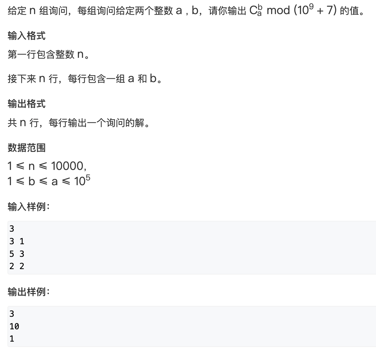
观察到数据范围到了 1 0 5 10 ^ 5 105级别, 直接使用递推***超时, 可以预处理阶乘和逆元, 利用组合数公式计算, 算法时间复杂度 O ( n log n ) O(n \log n) O(nlogn)
#include <bits/stdc++.h>

using namespace std;

typedef long long LL;
const int N = 1e5 + 10, MOD = 1e9 + 7;

int n;
LL fact[N], infact[N];

LL pow(LL a, LL b, LL p) {

    LL res = 1 % p;
    while (b) {

        if (b & 1) res = res * a % p;
        b >>= 1;
        a = a * a % p;
    }
    return res;
}

void init() {

    fact[0] = infact[0] = 1;
    for (int i = 1; i < N; ++i) {

        fact[i] = (LL) fact[i - 1] * i % MOD;
        infact[i] = pow(fact[i], MOD - 2, MOD);
    }
}

LL C(int a, int b) {

    LL res = fact[a] % MOD * infact[a - b] % MOD * infact[b] % MOD;
    return res;
}

int main() {

    ios::sync_with_stdio(false);
    cin.tie(0), cout.tie(0);

    init();

    int n;
    cin >> n;
    while (n--) {

        int a, b;
        cin >> a >> b;
        cout << C(a, b) << '\n';
    }

    return 0;
}
车的放置
序列统计
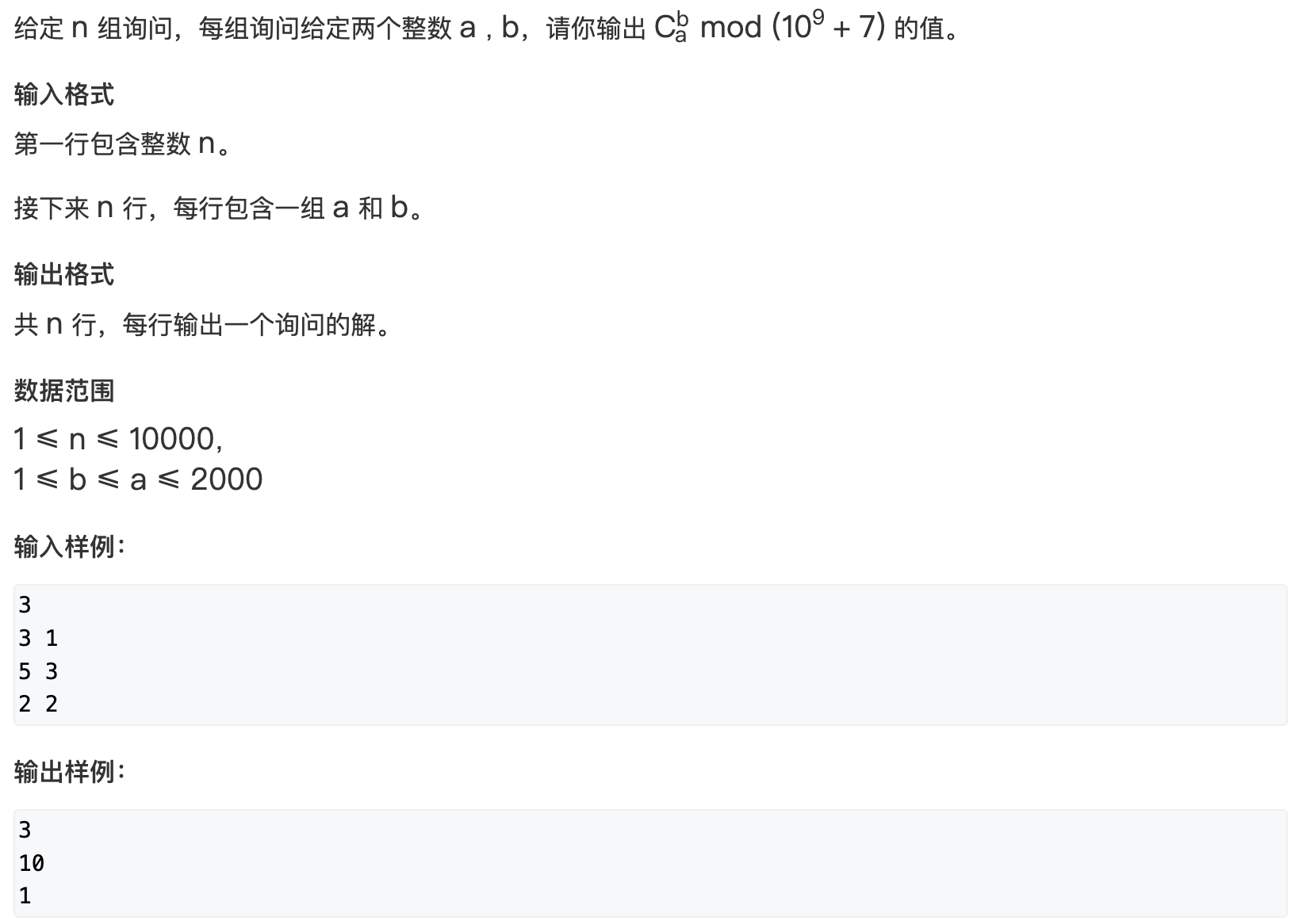
l u c a s lucas lucas定理求组合数 (数据范围非常大)
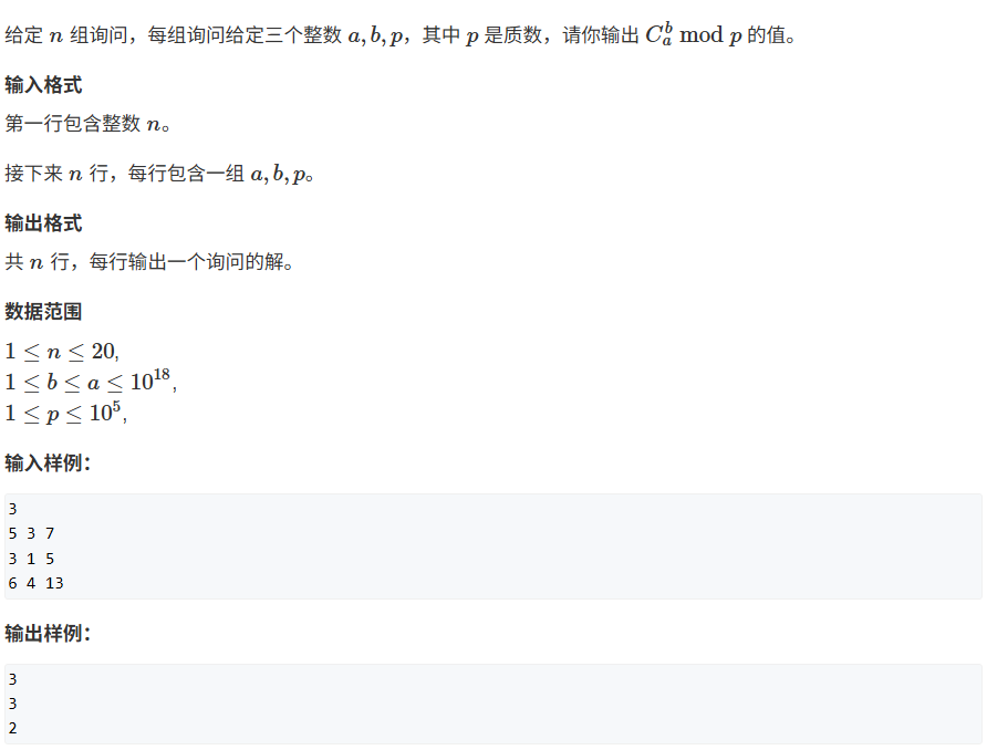
p p p的范围比较小 1 0 5 10 ^ 5 105, C a b ≡ C a m o d p b m o d p ⋅ C a p b p ( m o d p ) C_{a} ^ b \equiv C_{a \mod p} ^ {b \mod p} \cdot C_{\frac{a}{p}} ^ {\frac{b}{p}} (\mod p) Cab≡Camodpbmodp⋅Cpapb(modp), 时间复杂度 O ( log p N ⋅ p ⋅ log p ) O(\log _{p} ^ N \cdot p \cdot \log_p) O(logpN⋅p⋅logp), 计算每一项组合数除法部分使用乘法逆元
引理
引理1: C p x ≡ 0 ( m o d p ) , ( 0 < x < p ) C_{p} ^ x \equiv 0 (\mod p), (0 < x < p) Cpx≡0(modp),(0<x<p)
C p x = p ! x ! ( p − x ) ! = p x ⋅ ( p − 1 ) ! ( x − 1 ) ! ( p − x ) ! = p x ⋅ C p − 1 x − 1 C_{p} ^ x = \frac{p!}{x!(p - x)!} = \frac{p}{x}\cdot \frac{(p - 1)!}{(x - 1)!(p - x)!} = \frac{p}{x} \cdot C_{p - 1} ^ {x - 1} Cpx=x!(p−x)!p!=xp⋅(x−1)!(p−x)!(p−1)!=xp⋅Cp−1x−1
C p x ≡ 0 ( m o d p ) , ( 0 < x < p ) C_{p} ^ x \equiv 0 (\mod p), (0 < x < p) Cpx≡0(modp),(0<x<p)
引理 2 2 2: ( 1 + x ) p ≡ 1 + x p ( m o d p ) (1 + x) ^ p \equiv 1 + x ^ p (\mod p) (1+x)p≡1+xp(modp), 由二项式定理可知 ( 1 + x ) p = ∑ i = 0 p C p i x i (1 + x) ^ p = \sum_{i = 0} ^ p C_{p} ^ ix ^i (1+x)p=∑i=0pCpixi
因为 0 < x < p 0 < x < p 0<x<p, 因此上述二项式定理展开只剩 C p 0 C_p ^ 0 Cp0和 C p p C_p ^ p Cpp项, 也就是 1 + x p 1 + x ^ p 1+xp, 证毕
l u c a s lucas lucas定理的证明
假设计算 C n m m o d p C_n ^ m \mod p Cnmmodp, 其中 n = a p + r 1 n = ap + r_1 n=ap+r1, m = c p + r 2 m = cp + r_2 m=cp+r2
式子(1): ( 1 + x ) n = ∑ i = 0 p C n i x i ( m o d p ) (1 + x) ^ n = \sum_{i = 0} ^ p C_{n} ^ ix ^ i (\mod p) (1+x)n=∑i=0pCnixi(modp)
式子(2): ( 1 + x ) n = ( 1 + x ) a p + r 1 = ( ( 1 + x ) a ) p ⋅ ( 1 + x ) r 1 = ( 1 + x ) p a ⋅ ( 1 + x ) r 1 (1 + x) ^ n = (1 + x) ^ {ap + r1} = ((1 + x) ^ a) ^ p \cdot (1 + x) ^ {r_1} = (1 + x) ^ {pa} \cdot (1 + x) ^ {r_1} (1+x)n=(1+x)ap+r1=((1+x)a)p⋅(1+x)r1=(1+x)pa⋅(1+x)r1
根据引理(1), 式子(2) = ( 1 + x p ) a ⋅ ( 1 + x ) r 1 (1 + x ^ p) ^ {a} \cdot (1 + x) ^ {r_1} (1+xp)a⋅(1+x)r1, 将该式子用二项式定理展开
∑ i = 0 a C a i x i p ⋅ ∑ i = 0 r 1 C r 1 i x i \sum_{i = 0} ^ a C_a ^ ix ^ {ip} \cdot \sum_{i = 0} ^ {r_1} C_{r_1} ^ i x ^ i ∑i=0aCaixip⋅∑i=0r1Cr1ixi
假设当前 i = m i = m i=m, 观察式子(1)的 x m x ^ m xm项的系数是 C n m C_n ^ m Cnm
因为我们假设了 m = c p + r 2 m = cp + r_2 m=cp+r2, x m = x c p + r 2 = x c p ⋅ x r 2 x ^ m = x ^ {cp + r_2} = x ^ {cp} \cdot x ^ {r_2} xm=xcp+r2=xcp⋅xr2, 因此(2)式子的系数是 C a c ⋅ C r 1 r 2 C_a ^ c \cdot C_{r_1} ^ {r_2} Cac⋅Cr1r2
因为式子(1) = 式子(2), 同一项的系数相等, 因此 C n m = C a c ⋅ C r 1 r 2 C_n ^ m = C_a ^ c \cdot C_{r_1} ^ {r_2} Cnm=Cac⋅Cr1r2
因为 n n n和 m m m可以表示为 n = a p + r 1 n = ap + r_1 n=ap+r1, m = c p + r 2 m = cp + r_2 m=cp+r2
因此 C n m ≡ C n p m p ⋅ C n m o d p m m o d p ( m o d p ) C_{n} ^ m \equiv C_{\frac{n}{p}} ^ {\frac{m}{p}} \cdot C_{n \mod p} ^ {m \mod p} (\mod p) Cnm≡Cpnpm⋅Cnmodpmmodp(modp), 证毕
递归的边界是 b p = 0 \frac{b}{p} = 0 pb=0的时候, 返回 1 1 1
#include <bits/stdc++.h>

using namespace std;

typedef long long LL;
const int N = 1e5 + 10;

LL fact[N],  infact[N];

LL pow(LL a, LL b, LL p) {

    LL res = 1 % p;
    while (b) {

        if (b & 1) res = res * a % p;
        b >>= 1;
        a = a * a % p;
    }
    return res;
}

LL get(LL a, LL b, LL p) {

    memset(fact, 0, sizeof fact);
    memset(infact, 0, sizeof infact);
    fact[0] = infact[0] = 1;
    for (int i = 1; i <= a; ++i) {

        fact[i] = fact[i - 1] * i % p;
        infact[i] = pow(fact[i], p - 2, p);
    }
    LL res = fact[a] % p * infact[b] % p * infact[a - b] % p;
    return res;
}

LL lucas(LL a, LL b, LL p) {

    if (b == 0) return 1;
    return lucas(a / p, b / p, p) * get(a % p, b % p, p) % p;
}

int main() {

    ios::sync_with_stdio(false);
    cin.tie(0), cout.tie(0);

    int n;
    cin >> n;
    while (n--) {

        LL a, b, p;
        cin >> a >> b >> p;
        cout << lucas(a, b, p) << '\n';
    }

    return 0;
}
高精度求组合数(不取模)
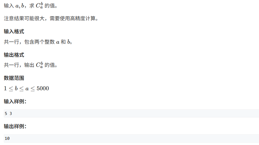
根据组合数定义 C n m = n ! m ! ( n − m ) ! C_n ^ m = \frac{n!}{m!(n - m)!} Cnm=m!(n−m)!n!, 如果直接计算高精度乘法和除法, 时间复杂度较高, 可以做如下考虑
将所有阶乘分解质因数, 结果的每个质因子出现的个数等于分子出现的次数 - 分母出现的次数, 假设对每个数字分解质因数, 算法时间复杂度 O ( n n ) O(n \sqrt n) O(nn), 还是无法接受的, 做如下优化:
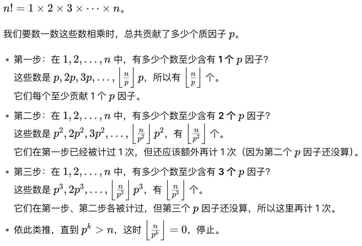
预处理数据范围内的所有质数, 计算每个阶乘内该质数出现的次数(勒让德公式), c n t = ⌊ n p ⌋ + ⌊ n p 2 ⌋ + ⌊ n p 3 ⌋ + . . . + ⌊ n p k ⌋ cnt = \left \lfloor \frac{n}{p} \right \rfloor + \left \lfloor \frac{n}{p ^ 2} \right \rfloor + \left \lfloor \frac{n}{p ^ 3} \right \rfloor + ... + \left \lfloor \frac{n}{p ^ k} \right \rfloor cnt=⌊pn⌋+⌊p2n⌋+⌊p3n⌋+...+⌊pkn⌋, 在算法实现过程中, 可以先计算 n b \frac{n}{b} bn, 然后迭代 n n n, 这样就能筛出 p 2 , p 3 , p 4 , . . . p ^ 2, p ^ 3, p ^ 4, ... p2,p3,p4,...的出现的次数
高精度部分只需要实现高精度乘法
#include <bits/stdc++.h>

using namespace std;

typedef long long LL;

const int N = 5010;

int cnt, primes[N];
bool st[N];
LL sum[N];

void init() {

    for (int i = 2; i < N; ++i) {

        if (!st[i]) primes[cnt++] = i;
        for (int j = 0; i * primes[j] < N; ++j) {

            st[i * primes[j]] = true;
            if (i % primes[j] == 0) break;
        }
    }
}

LL get(int n, int val) {

    LL res = 0;
    while (n) {

        res += n / val;
        n /= val;
    }
    return res;
}

vector<int> mul(vector<int> &a, int b) {

    vector<int> res;
    LL c = 0;
    for (int i = 0; i < a.size(); ++i) {

        c += a[i] * b;
        res.push_back(c % 10);
        c /= 10;
    }
    while (c) res.push_back(c % 10), c /= 10;
    return res;
}
int main() {

    ios::sync_with_stdio(false);
    cin.tie(0);

    init();

    int a, b;
    cin >> a >> b;
    for (int i = 0; i < cnt; ++i) {

        int val = primes[i];
        sum[i] = get(a, val) - get(b, val) - get(a - b, val);
    }

    vector<int> res(1, 1);
    for (int i = 0; i < cnt; ++i) {

        for (int j = 0; j < sum[i]; ++j) {

            res = mul(res, primes[i]);
        }
    }

    for (int i = res.size() - 1; i >= 0; --i) cout << res[i];
    cout << '\n';

    return 0;
}
不进行优化的高精度乘除法运算
高精度除法
#include <bits/stdc++.h>

using namespace std;

vector<int> res;

void div(vector<int> &d, int val, int &r) {

    r = 0;
    for (int i = d.size() - 1; i >= 0; --i) {

        r = r * 10 + d[i];
        res.push_back(r / val), r %= val;
    }

    reverse(res.begin(), res.end());
    while (res.size() > 1 && res.back() == 0) res.pop_back();
}

int main() {

    ios::sync_with_stdio(false);
    cin.tie(0);

    string s;
    int val;
    cin >> s >> val;

    int r;
    vector<int> d;
    for (int i = s.size() - 1; i >= 0; --i) d.push_back(s[i] - '0');

    div(d, val, r);

    for (int i = res.size() - 1; i >= 0; --i) cout << res[i];
    cout << '\n';
    cout << r << '\n';
    return 0;
}
(Catalan序列)满足条件的 01 01 01序列
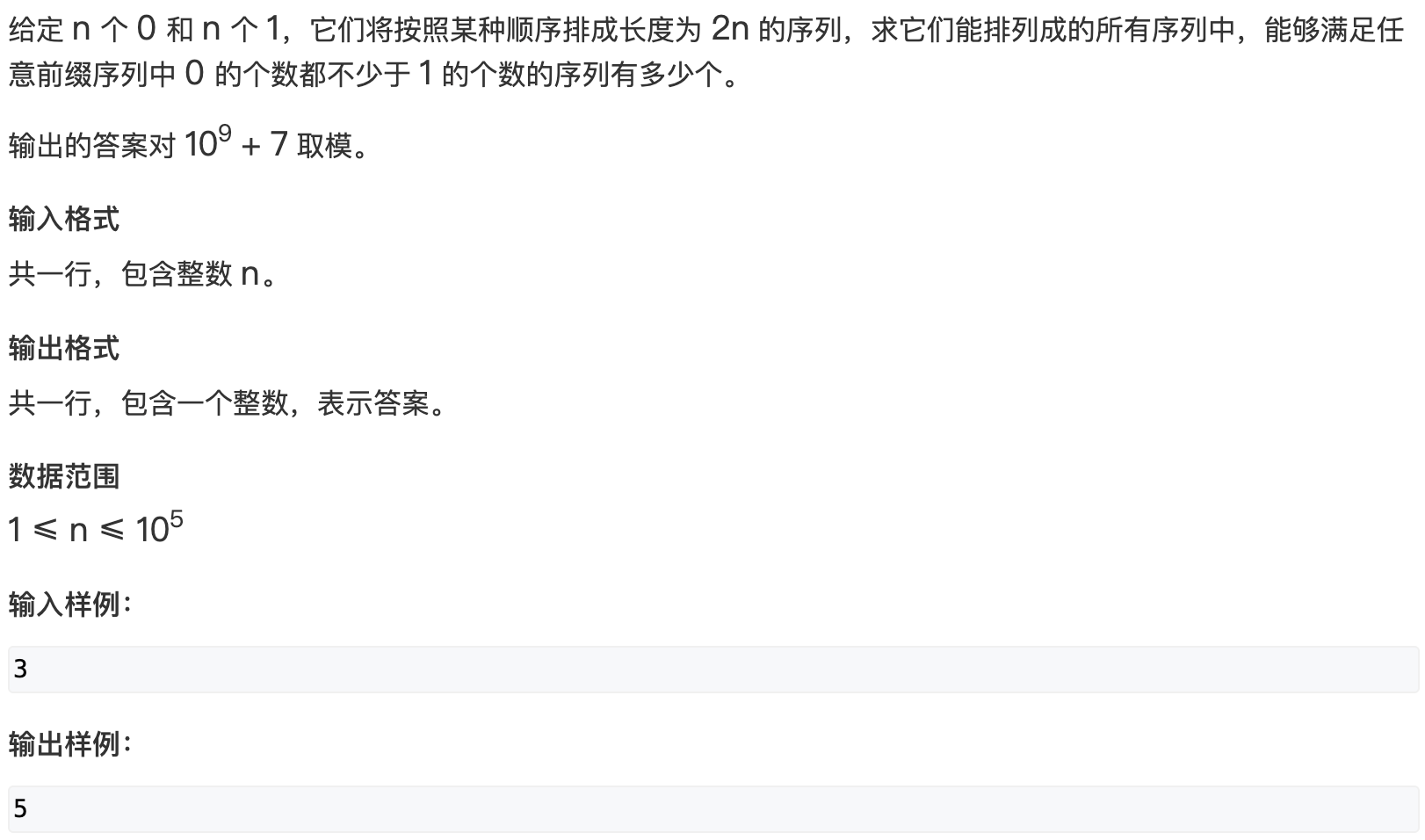
将向右走看作 0 0 0, 向上走看作 1 1 1
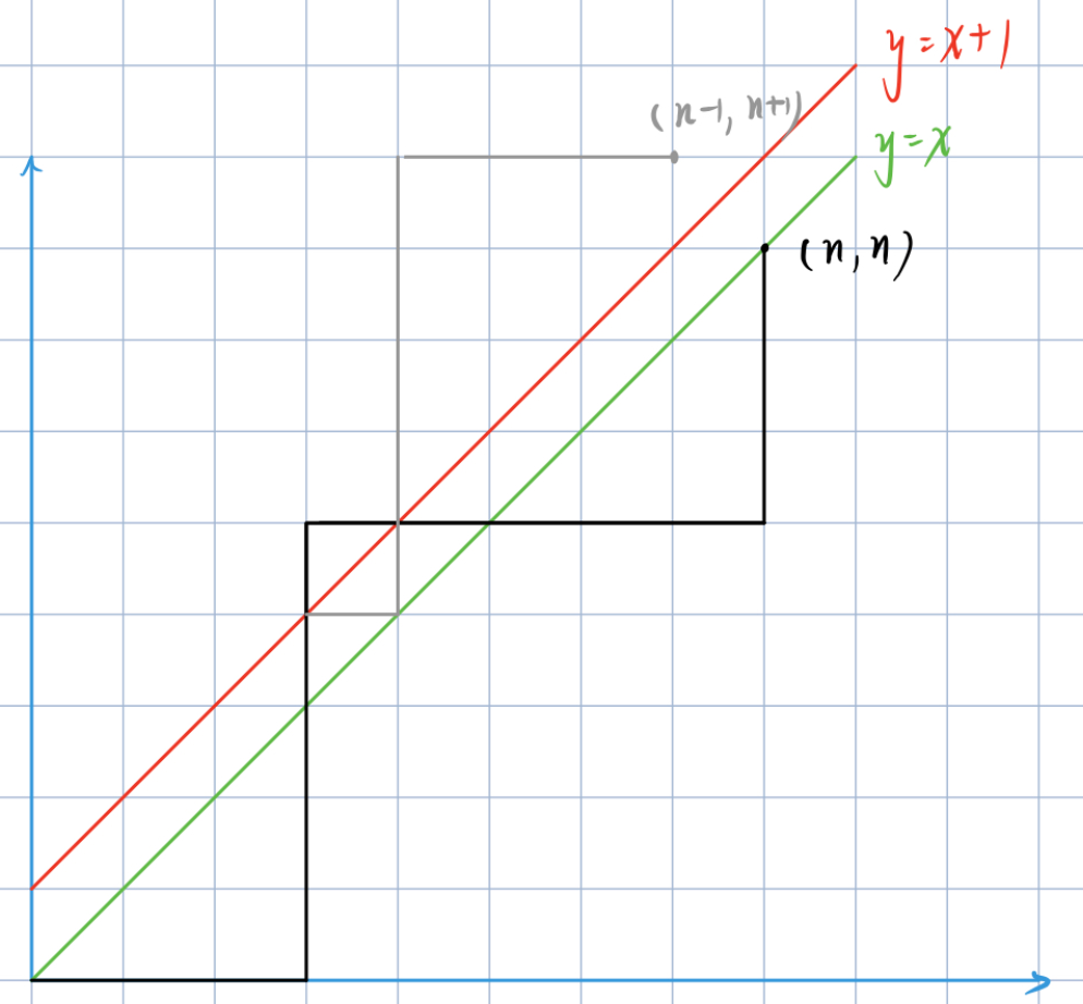
结果就是从起点 ( 0 , 0 ) (0, 0) (0,0)向上走到 ( n , n ) (n, n) (n,n)的合法的方案数量, 路线走到红颜色线就是非法的, 上述黑色的路径就是非法的, 注意观察所有的非法路径, 因为路径一定初始经过红色线, 然后再离开红色线
将经过红色线的部分按照红色线进行翻转(翻转是为了方便计算, 并且翻转后的路径和反转前的路径长度一致), 最终的终点都是 ( n − 1 , n + 1 ) (n - 1, n + 1) (n−1,n+1), 非法的方案数 C 2 n n − 1 C_{2n} ^ {n - 1} C2nn−1
最终的答案 a n s = C 2 n n − C 2 n n − 1 ans = C_{2n} ^ n - C_{2n} ^ {n - 1} ans=C2nn−C2nn−1, 数据范围 1 0 5 10 ^ 5 105, 可以使用快速幂求逆元的方式计算组合数, 算法时间复杂度 O ( n log n ) O(n \log n) O(nlogn)
#include <bits/stdc++.h>

using namespace std;

typedef long long LL;
const int N = 2e5 + 10, MOD = 1e9 + 7;

LL fact[N], infact[N];

LL pow(LL a, LL b, LL p) {

    LL res = 1 % p;
    a %= p;
    while (b) {

        if (b & 1) res = res * a % p;
        a = a * a % p;
        b >>= 1;
    }
    return res;
}

void init() {

    fact[0] = infact[0] = 1;
    for (int i = 1; i < N; ++i) {

        fact[i] = fact[i - 1] * i % MOD;
        infact[i] = pow(fact[i], MOD - 2, MOD);
    }
}

LL get(int a, int b) {

    if (a < b) return 0;
    return fact[a] * infact[a - b] % MOD * infact[b] % MOD;
}

int main() {

    ios::sync_with_stdio(false);
    cin.tie(0);

    init();

    int n;
    cin >> n;

    LL c1 = get(2 * n, n);
    LL c2 = get(2 * n, n - 1);

    LL res = (c1 - c2 + MOD) % MOD;

    cout << res << '\n';
    return 0;
}
网格
有趣的数列
容斥原理
韦恩图
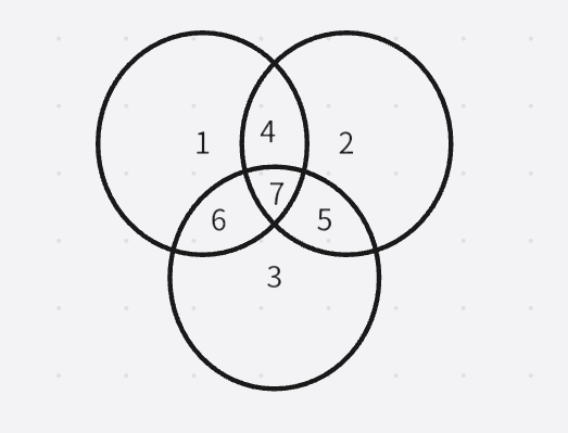
实际的面积等于 ∣ S 1 ∪ S 2 ∪ S 3 ∣ = ∣ S 1 ∣ + ∣ S 2 ∣ + ∣ S 3 ∣ − ∣ S 1 ∩ S 2 ∣ − ∣ S 2 ∩ S 3 ∣ − ∣ S 1 ∩ S 3 ∣ + ∣ S 1 ∩ S 2 ∩ S 3 ∣ |S_1 \cup S_2 \cup S_3| = |S_1| + |S_2| + |S_3| - |S_1 \cap S_2| - |S_2 \cap S_3| - |S_1 \cap S_3| + |S_1 \cap S_2 \cap S_3| ∣S1∪S2∪S3∣=∣S1∣+∣S2∣+∣S3∣−∣S1∩S2∣−∣S2∩S3∣−∣S1∩S3∣+∣S1∩S2∩S3∣
推广到 n n n个圆的面积, 下面的数字代表组合
1 − 2 + 3 − 4 + 5 − 6 + . . . 1 - 2 + 3 - 4 + 5 - 6 + ... 1−2+3−4+5−6+...
上述式子的项数的个数 C n 1 + C n 2 + C n 3 + . . . + C n n = C n 0 + C n 1 + C n 2 + C n 3 + . . . + C n n − 1 C_{n} ^ 1 + C_{n} ^ {2} + C_{n} ^ 3 + ... + C_{n} ^ {n} = C_{n} ^ 0 + C_{n} ^ 1 + C_{n} ^ {2} + C_{n} ^ 3 + ... + C_{n} ^ {n} - 1 Cn1+Cn2+Cn3+...+Cnn=Cn0+Cn1+Cn2+Cn3+...+Cnn−1
相当于从 n n n个数中挑任意多个数字的方案数, 实际等于 2 n − 1 2 ^ n - 1 2n−1项, 时间复杂度 O ( 2 n ) O(2 ^ n) O(2n)
能被整除的数
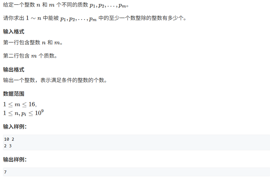
如果直接暴力做该问题, 算法时间复杂度 O ( n m ) O(nm) O(nm), 容斥原理时间复杂度 O ( 2 m ) O(2 ^ m) O(2m)
#include <bits/stdc++.h>

using namespace std;

typedef long long LL;
const int N = 20;

int n, m;
int p[N];

int main() {

    ios::sync_with_stdio(false);
    cin.tie(0), cout.tie(0);

    cin >> n >> m;
    for (int i = 0; i < m; ++i) cin >> p[i];

    LL res = 0;
    // 因为至少选择一个, 因此从1开始
    for (int i = 1; i < 1 << m; ++i) {

        LL tmp = 1, cnt = 0;
        for (int j = 0; j < m; ++j) {

            if (i >> j & 1) {

                if ((LL) tmp * p[j] > n) {

                    tmp = -1;
                    break;
                }
                tmp = tmp * p[j];
                cnt++;
            }
        }
        if (tmp != -1) (cnt & 1) ? res += n / tmp : res -= n / tmp;
    }

    cout << res << '\n';

    return 0;
}
Devu和鲜花
M o ¨ b i u s Möbius Mo¨bius函数
假设对数字 x x x分解质因数的结果是 p 1 α 1 p 2 α 2 . . . p k α k p_1 ^ {\alpha_1}p_2^ {\alpha_2}...p_k ^ {\alpha_k} p1α1p2α2...pkαk
μ ( x ) = { 0 α i > 1 1 k m o d 2 = 0 , α i = 1 − 1 k m o d 2 = 1 , α i = 1 \mu (x) = \begin{cases} 0 \; \; \; \; \; \; \; \; \; \; \alpha_i > 1\\ 1 \; \; \; \; \; \; \; \; \; \; k \mod 2 = 0, \alpha_i = 1\\ -1 \; \; \; \; \; \; \; k \mod 2 = 1, \alpha_i = 1 \end{cases} μ(x)=⎩ ⎨ ⎧0αi>11kmod2=0,αi=1−1kmod2=1,αi=1
破译密码
概率与数学期望
假设 a a a事件发生的概率是 X X X, b b b事件发生的概率是 Y Y Y, 那么有
E ( a X + b Y ) = a ⋅ E ( X ) + b ⋅ E ( Y ) E(aX + bY) = a \cdot E(X) +b \cdot E(Y) E(aX+bY)=a⋅E(X)+b⋅E(Y)
可以独立计算 E ( X ) E(X) E(X)和 E ( Y ) E(Y) E(Y)
扑克牌
绿豆蛙的归宿
博弈论
NIM游戏
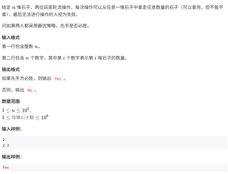
引理: a 1 ⊕ a 2 ⊕ a 3 ⊕ . . . ⊕ a n = 0 a_1 \oplus a_2 \oplus a_3 \oplus ... \oplus a_n = 0 a1⊕a2⊕a3⊕...⊕an=0, 先手必败
首先证明从 a 1 ⊕ a 2 ⊕ a 3 ⊕ . . . ⊕ a n ≠ 0 a_1 \oplus a_2 \oplus a_3 \oplus ... \oplus a_n \ne 0 a1⊕a2⊕a3⊕...⊕an=0的状态一定能通过某种方式转移到 a 1 ⊕ a 2 ⊕ a 3 ⊕ . . . ⊕ a n = 0 a_1 \oplus a_2 \oplus a_3 \oplus ... \oplus a_n = 0 a1⊕a2⊕a3⊕...⊕an=0状态
首先是最终状态没有石子, 0 ⊕ 0 = 0 0 \oplus 0 = 0 0⊕0=0
然后讨论 a 1 ⊕ a 2 ⊕ a 3 ⊕ . . . ⊕ a n = x ≠ 0 a_1 \oplus a_2 \oplus a_3 \oplus ... \oplus a_n = x \ne 0 a1⊕a2⊕a3⊕...⊕an=x=0的情况, 一定可以通过某种方式使得 x x x变为 0 0 0
假设 x x x的二进制表示中最高位的一个 1 1 1在第 k k k位置, a 1 , a 2 , a 3 , a n a_1, a_2, a_3, a_n a1,a2,a3,an中存在一个数字的第 k k k位是 1 1 1(反证法证明)
因为 x x x的最高位是 1 1 1, 显然有 a i ⊕ x < a i a_i \oplus x < a_i ai⊕x<ai, 可以从 a i a_i ai中拿出 a i − ( a i ⊕ x ) a_i - (a_i \oplus x) ai−(ai⊕x)这些石子, 剩余石子是 a i ⊕ x a_i \oplus x ai⊕x
因为拿走之前的数字异或值是 a 1 ⊕ a 2 ⊕ a 3 ⊕ . . . ⊕ { a i ⊕ x } ⊕ a n = x ⊕ x = 0 a_1 \oplus a_2 \oplus a_3 \oplus ... \oplus \{a_i \oplus x \}\oplus a_n = x \oplus x = 0 a1⊕a2⊕a3⊕...⊕{ ai⊕x}⊕an=x⊕x=0
因此一定存在某种方式使得 x ≠ 0 x \ne 0 x=0可以通过某种方式使得拿取石子之后 x x x变为 0 0 0
再证明 a 1 ⊕ a 2 ⊕ a 3 ⊕ . . . ⊕ a n = 0 a_1 \oplus a_2 \oplus a_3 \oplus ... \oplus a_n = 0 a1⊕a2⊕a3⊕...⊕an=0无论通过任何方式一定都会转移到 a 1 ⊕ a 2 ⊕ a 3 ⊕ . . . ⊕ a n ≠ 0 a_1 \oplus a_2 \oplus a_3 \oplus ... \oplus a_n \ne 0 a1⊕a2⊕a3⊕...⊕an=0状态
反证法, 假设拿完石子后的状态是 a 1 ⊕ a 2 ⊕ a 3 ⊕ . . . ⊕ a i ′ ⊕ a n = x ⊕ x = 0 a_1 \oplus a_2 \oplus a_3 \oplus ... \oplus a_i' \oplus a_n = x \oplus x = 0 a1⊕a2⊕a3⊕...⊕ai′⊕an=x⊕x=0, 将原式每一项除了 a i a_i ai和 a i ′ a_i' ai′不进行异或操作, 得到的结果是 a i ′ ⊕ a i = 0 a_i' \oplus a_i = 0 ai′⊕ai=0, 因为拿的石子数量必须大于 0 0 0, 但是最后结果是 a i ′ = a i a_i' = a_i ai′=ai, 矛盾, 因此 a 1 ⊕ a 2 ⊕ a 3 ⊕ . . . ⊕ a n = 0 a_1 \oplus a_2 \oplus a_3 \oplus ... \oplus a_n = 0 a1⊕a2⊕a3⊕...⊕an=0状态一定会转移到 a 1 ⊕ a 2 ⊕ a 3 ⊕ . . . ⊕ a n ≠ 0 a_1 \oplus a_2 \oplus a_3 \oplus ... \oplus a_n \ne 0 a1⊕a2⊕a3⊕...⊕an=0状态
因为最终状态是 a 1 ⊕ a 2 ⊕ a 3 ⊕ . . . ⊕ a n ≠ 0 a_1 \oplus a_2 \oplus a_3 \oplus ... \oplus a_n \ne 0 a1⊕a2⊕a3⊕...⊕an=0, 并且从 a 1 ⊕ a 2 ⊕ a 3 ⊕ . . . ⊕ a n ≠ 0 a_1 \oplus a_2 \oplus a_3 \oplus ... \oplus a_n \ne 0 a1⊕a2⊕a3⊕...⊕an=0的状态一定能通过某种方式转移到 a 1 ⊕ a 2 ⊕ a 3 ⊕ . . . ⊕ a n = 0 a_1 \oplus a_2 \oplus a_3 \oplus ... \oplus a_n = 0 a1⊕a2⊕a3⊕...⊕an=0状态, 并且 a 1 ⊕ a 2 ⊕ a 3 ⊕ . . . ⊕ a n = 0 a_1 \oplus a_2 \oplus a_3 \oplus ... \oplus a_n = 0 a1⊕a2⊕a3⊕...⊕an=0状态只能转移到 a 1 ⊕ a 2 ⊕ a 3 ⊕ . . . ⊕ a n ≠ 0 a_1 \oplus a_2 \oplus a_3 \oplus ... \oplus a_n \ne 0 a1⊕a2⊕a3⊕...⊕an=0状态, 也就是 a 1 ⊕ a 2 ⊕ a 3 ⊕ . . . ⊕ a n = 0 a_1 \oplus a_2 \oplus a_3 \oplus ... \oplus a_n = 0 a1⊕a2⊕a3⊕...⊕an=0的状态永远都在对手侧, 因此先手必胜, 证毕
#include <bits/stdc++.h>

using namespace std;

int n;

int main() {

    ios::sync_with_stdio(false);
    cin.tie(0);

    cin >> n;
    int res = 0;
    for (int i = 0; i < n; ++i) {

        int val;
        cin >> val;
        res ^= val;
    }

    if (res == 0) cout << "No" << '\n';
    else cout << "Yes" << '\n';
    return 0;
}
台阶NIM游戏
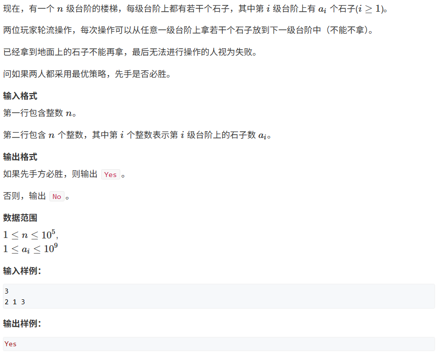
将奇数台阶上的石子看作经典 N i m Nim Nim游戏
证明:
先手状态 a 1 ⊕ a 3 ⊕ a 5 . . . ⊕ a k ≠ 0 a_1 \oplus a_3 \oplus a_5 ... \oplus a_k \ne 0 a1⊕a3⊕a5...⊕ak=0, 根据经典 N I m NIm NIm游戏, 存在一种方法使得将奇数台阶的石子异或值为 0 0 0, 也就是将该状态转移到后手
然后再看后手的情况
- 如果后手移动偶数台阶上的石子, 那么下一次先手只需要将上一次后手移动的石子顺次移动到奇数台阶上, 留给后手的局面还是奇数台阶上的石子异或值为 0 0 0
- 如果后手移动的是奇数台阶上的石子, 因为当前奇数台阶上的石子异或值为 0 0 0, 根据经典 N i m Nim Nim游戏, 后手移动之后, 奇数台阶上的石子异或值一定 ≠ 0 \ne 0 =0
因此, 奇数台阶石子异或值为 0 0 0的局面永远都在后手, 当所有奇数台阶上石子的数量为 0 0 0的时候, 需要移动偶数台阶上的石子
因为将偶数台阶上石子移动到地面需要的次数是偶数次!, 因此后手必败, 先手必胜, 证毕
#include <bits/stdc++.h>

using namespace std;

const int N = 1e5 + 10;

int n;

int main() {

    ios::sync_with_stdio(false);
    cin.tie(0);

    cin >> n;

    int res = 0;
    for (int i = 1; i <= n; ++i) {

        int val;
        cin >> val;
        if (i & 1) res ^= val;
    }

    cout << (res ? "Yes" : "No") << '\n';

    return 0;
}
S G SG SG函数
能解决大部分博弈论问题
定义 M e x ( i ) Mex(i) Mex(i)是集合 i i i中不存在的最小的自然数
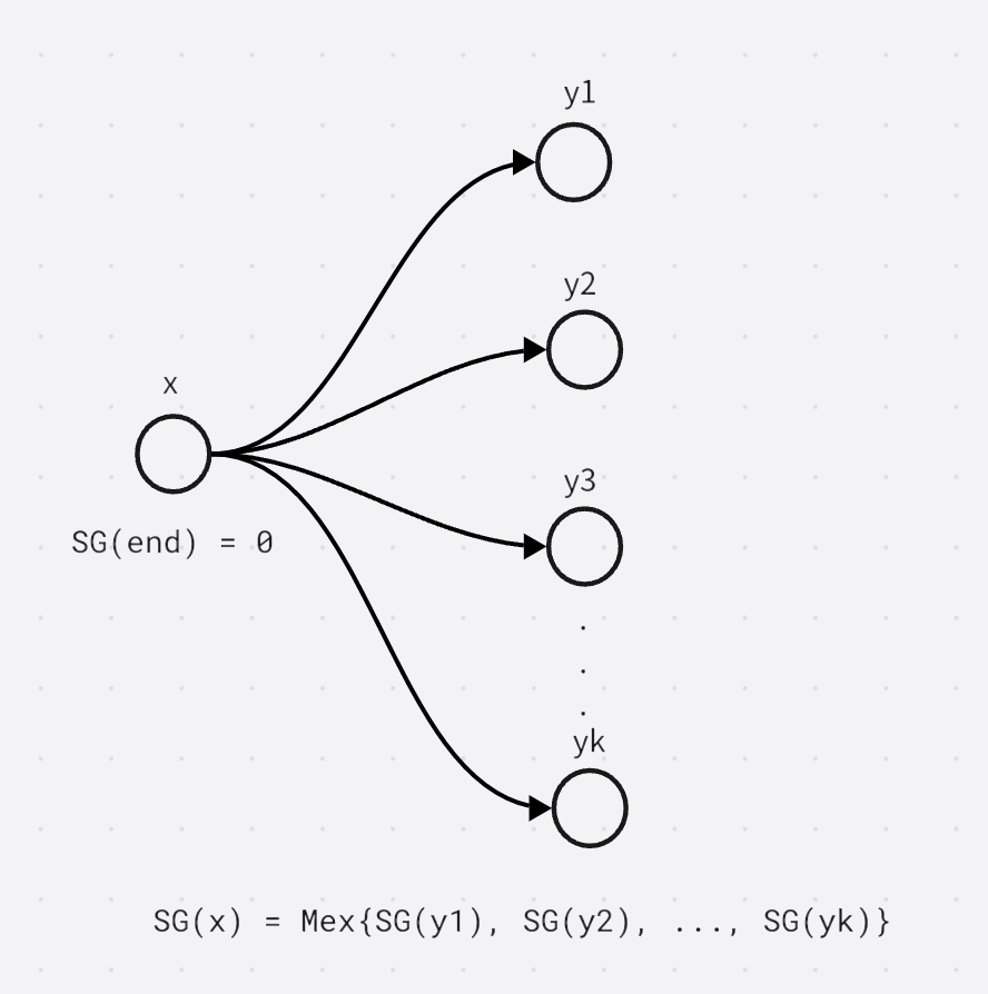
如果只有一个状态图, 如果 S G ( x ) = 0 SG(x) = 0 SG(x)=0必败, S G ( x ) ≠ 0 SG(x) \ne 0 SG(x)=0必胜, 也就是任何非零状态都能到 0 0 0, 任何 0 0 0状态只能到非零
如果有 n n n张图, 将所有起点的 S G SG SG值进行异或, 如果 = 0 = 0 =0必败, ≠ 0 \ne 0 =0必胜
证明方式类似于 N i m Nim Nim游戏, 还是从两方面证明, 证明略
集合NIM游戏(记忆化搜索实现 S G SG SG函数)
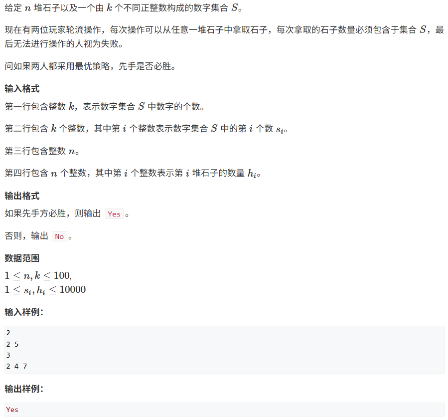
每次取的石子的数量限定在集合 S S S中
假设 S = { 2 , 5 } S = \{2, 5\} S={ 2,5}, 假设只有一堆石子, 石子的数量是 10 10 10
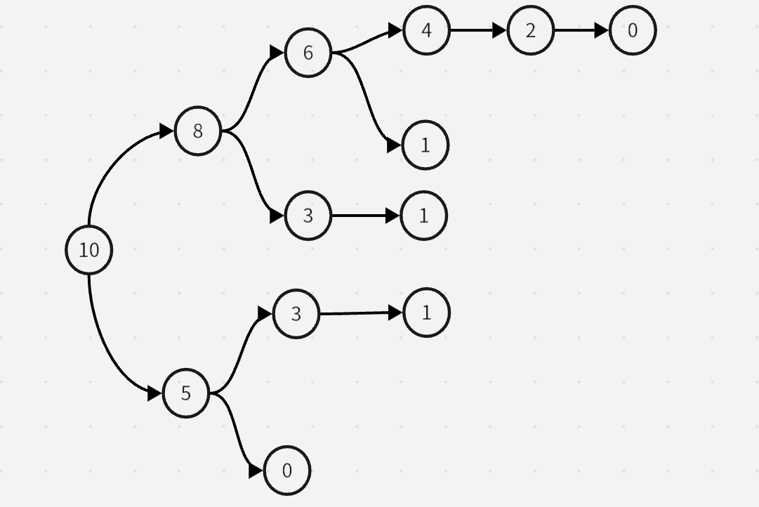
这样就可以从终点状态向前计算出初始状态的 S G SG SG的值, n n n堆石子可以看作 n n n个状态图, 然后计算每个图的初始状态的 S G SG SG值, 再异或
#include <bits/stdc++.h>

using namespace std;

const int N = 110, M = 10010;

int k, s[N];
int n;
int f[M];

int sg(int x) {

    if (f[x] != -1) return f[x];

    unordered_set<int> S;
    for (int i = 0; i < k; ++i) {

        if (x >= s[i]) S.insert(sg(x - s[i]));
    }

    for (int i = 0; ; ++i) {

        if (!S.count(i)) return f[x] = i;
    }
}

int main() {

    ios::sync_with_stdio(false);
    cin.tie(0), cout.tie(0);

    cin >> k;
    for (int i = 0; i < k; ++i) cin >> s[i];

    memset(f, -1, sizeof f);
    int res = 0;

    cin >> n;
    for (int i = 0; i < n; ++i) {

        int val;
        cin >> val;
        res ^= sg(val);
    }

    cout << (res ? "Yes" : "No") << '\n';
    return 0;
}
拆分NIM游戏

每次取走一堆石子, 然后放入两堆规模更小的石子
相较于集合 N i m Nim Nim游戏, 假设取走的石子数量是 a i a_i ai, 定义添加进来的两堆石子数量是 b i , b j b_i, b_j bi,bj, 规定 b i ≥ b j b_i \ge b_j bi≥bj(这样规定是为了不重复计算), 也就是将当前局面拆分为两个局面, 由 S G SG SG函数定义可知, 计算多个局面的 S G SG SG值就是将这些 S G SG SG进行异或
#include <bits/stdc++.h>

using namespace std;

const int N = 110;

int n, w[N];
int f[N];

int sg(int x) {

    if (f[x] != -1) return f[x];
    unordered_set<int> S;

    for (int i = 0; i < x; ++i) {

        for (int j = 0; j <= i; ++j) {

            S.insert(sg(i) ^ sg(j));
        }
    }
    for (int i = 0; ; ++i) {

        if (!S.count(i)) return f[x] = i;
    }
}

int main() {

    ios::sync_with_stdio(false);
    cin.tie(0);

    cin >> n;

    int res = 0;
    memset(f, -1, sizeof f);

    for (int i = 0; i < n; ++i) {

        int val;
        cin >> val;
        res ^= sg(val);
    }

    cout << (res ? "Yes" : "No") << '\n';

    return 0;
}

 京公网安备 11010502036488号