线性代数之——矩阵乘法和逆矩阵

1. 矩阵乘法

如果矩阵 $B$B 的列为 $b_1,b_2,b_3$b1​,b2​,b3​，那么 $EB$EB 的列就是 $E{b}_1,E{b}_2,E{b}_3$Eb1​,Eb2​,Eb3​。

$EB=E\left[b_1{b}_2{b}_3\right]=\left[E{b}_{1}E{b}_{2}E{b}_3\right]$EB=E[b1​b2​b3​]=[Eb1​Eb2​Eb3​]

$E\left(B的第j列\right)=EB的第j列$E (B的第 j 列)=EB 的第 j 列

• 置换矩阵（permutation matrix）

在消元的过程中，如果遇到了某一行主元的位置为 0，而其下面一行对应的位置不为 0，我们就可以通过行交换来继续进行消元。

如下的矩阵 $P_{23}$P23​ 可以实现将向量或者矩阵的第 2 、 3 行进行交换。

$P_{23}=\left[\begin{array}{ccc}1& 0& 0\\ 0& 0& 1\\ 0& 1& 0\end{array}\right]$P23​=⎣⎡​100​001​010​⎦⎤​

$\left[\begin{array}{ccc}1& 0& 0\\ 0& 0& 1\\ 0& 1& 0\end{array}\right]\left[\begin{array}{c}1\\ 3\\ 5\end{array}\right]=\left[\begin{array}{c}1\\ 5\\ 3\end{array}\right]$⎣⎡​100​001​010​⎦⎤​⎣⎡​135​⎦⎤​=⎣⎡​153​⎦⎤​

$\left[\begin{array}{ccc}1& 0& 0\\ 0& 0& 1\\ 0& 1& 0\end{array}\right]\left[\begin{array}{ccc}2& 4& 1\\ 0& 0& 3\\ 0& 6& 5\end{array}\right]=\left[\begin{array}{ccc}2& 4& 1\\ 0& 6& 5\\ 0& 0& 3\end{array}\right]$⎣⎡​100​001​010​⎦⎤​⎣⎡​200​406​135​⎦⎤​=⎣⎡​200​460​153​⎦⎤​

置换矩阵 $P_{ij}$Pij​ 就是将单位矩阵的第 $i$i 行和第 $j$j 行进行互换，当交换矩阵乘以另一个矩阵时，它的作用就是交换那个矩阵的第 $i$i 行和第 $j$j 行。

• 增广矩阵（augmented matrix）

在消元的过程中，方程两边的系数 $A$A 和 $b$b 都要进行同样的变换，这样，我们可以把 $b$b 作为矩阵 $A$A 的额外的一列，然后，就可以用消元矩阵 $E$E 乘以这个增广的矩阵一次性完成左右两边的变换。

$E\left[Ab\right]=\left[EAEb\right]$E[A b]=[EA Eb]

$\left[\begin{array}{ccc}1& 0& 0\\ -2& 1& 0\\ 0& 0& 1\end{array}\right]\left[\begin{array}{cccc}2& 4& -2& 2\\ 4& 9& -3& 8\\ -2& -3& 7& 10\end{array}\right]=\left[\begin{array}{cccc}2& 4& -2& 2\\ 0& 1& 1& 4\\ -2& -3& 7& 10\end{array}\right]$⎣⎡​1−20​010​001​⎦⎤​⎣⎡​24−2​49−3​−2−37​2810​⎦⎤​=⎣⎡​20−2​41−3​−217​2410​⎦⎤​

• 矩阵乘法的四种理解

如果矩阵 $A$A 有 $n$n 列， $B$B 有 $n$n 行，那么我们可以进行矩阵乘法 $AB$AB。

假设矩阵 $A$A 有 $m$m 行 $n$n 列，矩阵 $B$B 有 $n$n 行 $p$p 列，那么 $AB$AB 是 $m$m 行 $p$p 列的。

$(m\times n)(n\times p)(m\times p)\left[\begin{array}{c}m行\\ n列\end{array}\right]\left[\begin{array}{c}n行\\ p列\end{array}\right]\left[\begin{array}{c}m行\\ p列\end{array}\right]$(m×n)(n×p)(m×p)[m 行n 列​][n 行p 列​][m 行p 列​]

矩阵乘法的第一种理解方式就是一个一个求取矩阵 $AB$AB 位于 $(i,j)$(i,j) 处的元素

$(AB{)}_{ij}=A的第i行与B的第j列的内积=\sum a_{ik}{b}_{kj}$(AB)ij​=A 的第 i 行与 B 的第 j 列的内积=∑aik​bkj​

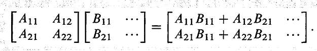
第二种理解，矩阵 $AB$AB 的列是 $A$A 的列的线性组合

$AB=A[b_1{b}_2\cdots b_p]=[A{b}_{1}A{b}_2\cdots A{b}_p]$AB=A[b1​b2​⋯bp​]=[Ab1​Ab2​⋯Abp​]

第三种理解，矩阵 $AB$AB 的行是 $B$B 的行的线性组合

$AB=\left[\begin{array}{c}{a}_1\\ a_2\\ ⋮\\ a_m\end{array}\right]B=\left[\begin{array}{c}{a}_{1}B\\ a_{2}B\\ ⋮\\ a_{m}B\end{array}\right]$AB=⎣⎢⎢⎢⎡​a1​a2​⋮am​​⎦⎥⎥⎥⎤​B=⎣⎢⎢⎢⎡​a1​Ba2​B⋮am​B​⎦⎥⎥⎥⎤​

第四种理解，矩阵 $AB$AB 是所有 $A$A 的列与 $B$B 的行的乘积的和

$AB=[a_1{a}_2\cdots a_n]\left[\begin{array}{c}{b}_1\\ b_2\\ ⋮\\ b_n\end{array}\right]=\sum _{i=1}^n{a}_i{b}_i$AB=[a1​a2​⋯an​]⎣⎢⎢⎢⎡​b1​b2​⋮bn​​⎦⎥⎥⎥⎤​=i=1∑n​ai​bi​

其中，一列乘以一行称为外积（outer product），(n×1)(1×n)=(n, n)，结果为一个 n×n 的矩阵。
$\left[\begin{array}{cc}2& 7\\ 3& 8\\ 4& 9\end{array}\right]\left[\begin{array}{cc}1& 6\\ 0& 0\end{array}\right]=\left[\begin{array}{c}2\\ 3\\ 4\end{array}\right]\left[16\right]+\left[\begin{array}{c}7\\ 8\\ 9\end{array}\right]\left[00\right]=\left[\begin{array}{cc}2& 12\\ 3& 18\\ 4& 24\end{array}\right]$⎣⎡​234​789​⎦⎤​[10​60​]=⎣⎡​234​⎦⎤​[16]+⎣⎡​789​⎦⎤​[00]=⎣⎡​234​121824​⎦⎤​

• 矩阵乘法的性质

结合律： $A\left(BC\right)=\left(AB\right)C$A(BC)=(AB)C
交换律： $(A+B)C=AC+BC$(A+B)C=AC+BC
交换律： $A(B+C)=AB+AC$A(B+C)=AB+AC

$A^p=\underset{\text{p 个}}{\underbracket{AA\cdots A}}$Ap=p 个 AA⋯A​​
$A^p{A}^q=A^{(p+q)}$ApAq=A(p+q)
$(A^p{)}^q=A^{pq}$(Ap)q=Apq
$A^0=I$A0=I

• 分块矩阵

矩阵还可以被划分为小块，其中每个小块都是一个更小的矩阵。

如果对矩阵 $A$A 的列的划分和对矩阵 $B$B 的行的划分正好匹配，那么每个块之间就可以进行矩阵乘法。

一种特殊的划分就是矩阵 $A$A 的每个小块都是 $A$A 的一列，矩阵 $B$B 的每个小块都是 $B$B 的一行，这种情况就是我们上面说的矩阵相乘的第四种理解。

同样地，在消元的时候，我们也可以按块对系数矩阵进行消元。

2. 矩阵的逆

假设 $A$A 是一个方阵，如果存在一个矩阵 $A^{-1}$A−1，使得

$A^{-1}A=I并且A{A}^{-1}=I$A−1A=I并且AA−1=I

那么，矩阵 $A$A 就是可逆的， $A^{-1}$A−1 称为 $A$A 的逆矩阵。

逆矩阵的逆就是进行和原矩阵相反的操作。消元矩阵 $E_{21}$E21​ 的作用是第二个方程减去第一个方程的 2 倍。

$E_{21}=\left[\begin{array}{ccc}1& 0& 0\\ -2& 1& 0\\ 0& 0& 1\end{array}\right]$E21​=⎣⎡​1−20​010​001​⎦⎤​

其逆矩阵 $E_{21}^{-1}$E21−1​ 的作用则是第二个方程加上第一个方程的 2 倍。

$E_{21}^{-1}=\left[\begin{array}{ccc}1& 0& 0\\ 2& 1& 0\\ 0& 0& 1\end{array}\right]$E21−1​=⎣⎡​120​010​001​⎦⎤​

• 当且仅当在消元过程中产生 $n$n 个主元的时候（允许行交换），矩阵 $A$A 的逆才存在。

• 矩阵 $A$A 不可能有两个不同的逆矩阵，左逆等于右逆。假设 $BA=I$BA=I， $AC=I$AC=I，那么一定有 $B=C$B=C。
  $B\left(AC\right)=\left(BA\right)C\to BI=IC\to B=C$B(AC)=(BA)C→BI=IC→B=C

• 如果矩阵 $A$A 是可逆的，那么 $Ax=b$Ax=b 有唯一解 $x=A^{-1}b$x=A−1b。

• 如果存在一个非零向量 $x$x 使得 $Ax=0$Ax=0，那么 $A$A 不可逆，因为没有矩阵可以将零向量变成一个非零向量。

$若A^{-1}存在，则x=A^{-1}0=0$若 A−1 存在，则 x=A−10=0

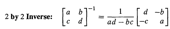
• 一个 2×2 的矩阵是可逆的，当且仅当 $ad-bc$ad−bc 非零。

• 一个对角化矩阵如果其对角线上元素非零，那么其有逆矩阵。

如果矩阵 $A$A 和矩阵 $B$B 都是可逆的，那么它们的乘积 $AB$AB 也是可逆的。

$(AB{)}^{-1}=B^{-1}{A}^{-1}$(AB)−1=B−1A−1
$(AB{)}^{-1}AB=B^{-1}{A}^{-1}AB=B^{-1}IB=I$(AB)−1AB=B−1A−1AB=B−1IB=I

同样地，针对三个或更多矩阵的乘积，有

$(ABC{)}^{-1}=C^{-1}{B}^{-1}{A}^{-1}$(ABC)−1=C−1B−1A−1

3. 高斯－若尔当消元法（Gauss-Jordan Elimination）求矩阵的逆

我们可以通过消元法来求解矩阵 $A$A 的逆矩阵。思路是这样的，假设 $A$A 是一个 3×3 的矩阵，那么我们可以建立三个方程来分别求出 $A^{-1}$A−1 的三列。

$A{A}^{-1}=A\left[x_1{x}_2{x}_3\right]=\left[e_1{e}_2{e}_3\right]=\left[\begin{array}{ccc}1& 0& 0\\ 0& 1& 0\\ 0& 0& 1\end{array}\right]$AA−1=A[x1​x2​x3​]=[e1​e2​e3​]=⎣⎡​100​010​001​⎦⎤​

$\begin{array}{c}{\displaystyle A{x}_1=e_1}\\ {\displaystyle A{x}_2=e_2}\\ {\displaystyle A{x}_3=e_3}\end{array}$Ax1​=e1​Ax2​=e2​Ax3​=e3​​

而高斯－若尔当消元法则是一次性求解出这些方程，之前我们求解一个方程的时候，将 $b$b 作为 $A$A 的一列组成增广矩阵，而现在我们则是把 $e_1、e_2、e_3$e1​、e2​、e3​ 三列一起放入 $A$A 中形成一个增广矩阵，然后进行消元。

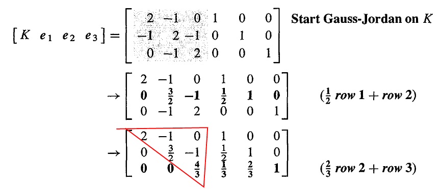
到这里，我们已经得到了一个下三角矩阵 $U$U，高斯就会停在这里然后用回带法求出方程的解，但若尔当将会继续进行消元，直到得到简化阶梯形式（reduced echelon form）。

最后，我们将每行都除以主元得到新的主元都为 1，此时，增广矩阵的前一半矩阵就是 $I$I，而后一半矩阵就是 $A^{-1}$A−1。

我们用分块矩阵就可以很容易地理解高斯－若尔当消元法，消元的过程就相当于乘以了一个 $A^{-1}$A−1 将 $A$A 变成了 $I$I，将 $I$I 变成了 $A^{-1}$A−1。

$A^{-1}\left[AI\right]=\left[I{A}^{-1}\right]$A−1[AI]=[IA−1]

获取更多精彩，请关注「seniusen」!