

概述
作者提出一种随即回答网络(stochastic answer network)来解决NLI问题.
和之前的模型根据输入直接预测结果不同, 该模型维护一个状态并迭代地改进其预测.
与单步推理相比, 这种多步推理方法可以对更复杂的推理任务进行建模.
模型
single-step inference architecture
单步推理网络结构就是利用输入的premise和hypothesis直接预测结果.
Multi-step inference with SAN
定义了一个新的循环状态 st, 模型在生成最终输出之前, 每个时间步迭代生成 st, 将 sT作为最终的输出.

模型结构分为四部分:
- Lexicon encoding layer: compute word representation
- contextual encoding layer: modifie word representation in context
- memory generation layer: gather information from premise and hypothesis, form a “working memory” for the final answer module
- final answer module: type of multi-step network, predicts the relation between the premise and hypothesis.
Lexicon Encoding layer
首先, 将词向量和字向量做拼接, 这样可以比较好的解决OOV问题.
之后将拼接向量输入到两层Position-wise前馈网络得到最终的lexicon embedding Ep∈Rd×m,Eh∈Rd×n.
Contextual Encoding layer
两层的BiLSTM
因为双向lstm输出是单向的2倍, 作者在每层LSTM加了maxout层来对BiLSTM进行压缩.
然后, 对两层LSTM的输出做一个拼接, 得到P和H的表示 Cp∈R2d×m,Ch∈R2d×n
Memory Layer
同样利用了注意力机制.
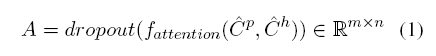
首先, 也是先进行向量点乘. 之后, 作者并没有对点乘结果进行softmax而是加了一层映射.
这里, A就是attention矩阵, C^p和 C^h是通过一层全连接 ReLU(W⋅x)得到的.
然后, 分别进行拼接
Up=[Cp;ChA] Uh=[Ch;CpA′]
接着,
Mp=BiLSTM([Up;Cp]) Mh=BiLSTM([Uh;Ch])
Answer module
answer module计算T个时间步的关系标签.
在最开始, 初始化状态 s0
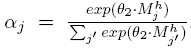
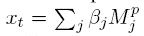
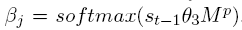
之后对于各个时间步的状态 st,
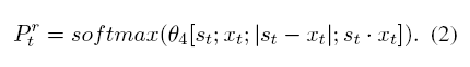
计算每个时间步的匹配结果 Ptr,
之后, 对各个时间步结果进行平均,
另外, 为了提高鲁棒性, 在训练期间使用stochastic prediction dropout.


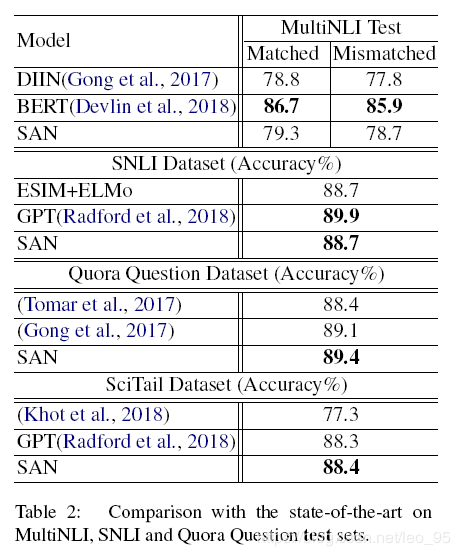
实验
实现细节
- 分词: spaCy
- word embedding: GloVe 300D
- character encoding: 利用CNN训练, embedding size设为20. windows设为1,3,5 hidden size设为50, 100, 150
- word embedding和character embedding拼接, 最终的lexicon embedding就是600维.
- LSTM hidden size: 128
- 注意力层的projection size: 256
- dropout: 0.2
- batch size: 32
- optimizer: Adamax
- learning rate: 0.002

 京公网安备 11010502036488号